suppressPackageStartupMessages(library(faux))
library(ggplot2)
options(digits = 3)

rsq <- function(f) summary(lm(f, data = pop))$r.squared

norm2negbin <- function (x, size, prob, mu = mean(x),
                         sd = stats::sd(x)) {
    p <- stats::pnorm(x, mu, sd)
    stats::qnbinom(p, size = size, prob = prob, mu = mu)
}

nice_n <- function (x) prettyNum(x, scientific = FALSE,
big.mark = ",")Correcting selection effects of noisy polygenic scores: an idiot’s guide
We’re interested in how natural selection is changing mean polygenic scores. In particular, we want to know how big the change is in one generation. We have at our disposal:
A dataset of individuals, with their polygenic score predicting (e.g.) educational attainment.
An estimate of the true heritability of educational attainment, perhaps from twin studies.
Data on the individuals’ relative lifetime reproductive success (RLRS; their number of children as a proportion of the average number of children in that generation). By definition this has a mean of 1.
We can estimate the effect of natural selection on polygenic scores by the Robertson-Price equation, which says:
Mean PGS in the children’s generation = Mean PGS in the parent’s generation plus covariance of PGS and RLRS.
We’re interested in the effect of natural selection on the true polygenic score – the best linear unbiased predictor of educational attainment, if we knew everyone’s genetic variants and had perfect estimates of their effect sizes. But we only have a noisy estimate of the true polygenic score!
Let’s simulate two generations, using the very helpful {faux} package by Lisa Debruine. First some useful functions:
Now we’ll create our data.
# I'll use a big sample to show that the estimates are indeed
# accurate "in the limit"
n <- 1e6

# For labels

# This is what we'd like to estimate:
selection_effect <- 0.1

# This is related to the variance of RLRS:
rlrs_dispersion <- 3

# Generate random variables: true PGS for educational attainment,
# Relative Lifetime Reproductive Success
pop <- faux::rmulti(n = n,
                    dist = c(pgs_true = "norm", rlrs = "norm",
                             pgs = "norm"),
                    params = list(
                                  pgs_true = list(mean = 0, sd = 1),
                                  rlrs = list(mean = 1, sd = 1)),
                    r = selection_effect)

pop$rlrs <- norm2negbin(pop$rlrs, mu = 1, size = rlrs_dispersion)
We can check our population parameters look right:
ggplot(pop, aes(rlrs)) +
  geom_bar(aes(y = after_stat(prop))) +
  theme_light() +
  labs(x = "RLRS", y= "Proportion of population")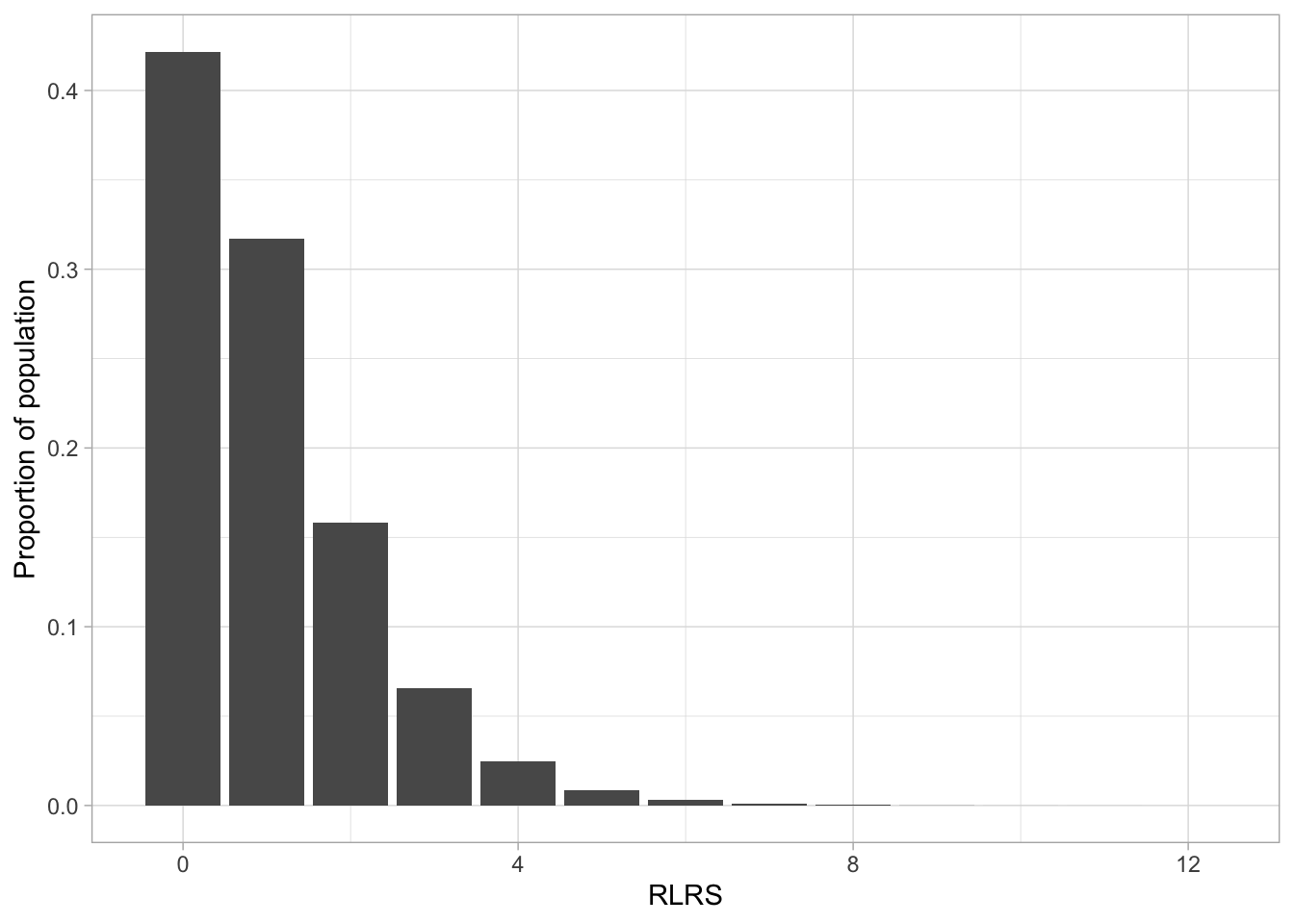
# Our PGS is normalized with mean 0 variance 1:
mean(pop$pgs_true)
[1] 0.000928var(pop$pgs_true)[1] 0.998# RLRS has mean 1:
mean(pop$rlrs)[1] 1# Covariance of RLRS with the true PGS:
cov(pop$pgs_true, pop$rlrs)[1] 0.104# and the mean pgs_true in the children's generation
# i.e. the change in one generation, measured in standard deviations:
weighted.mean(pop$pgs_true, pop$rlrs)[1] 0.105And here’s the plot:
ggplot(pop, aes(pgs_true, rlrs)) +
  geom_point(alpha = 0.05, pch = ".",
             position = position_jitter(height = 0.2)) +
  geom_smooth(method = "lm", formula = y~x, color = "red") +
  coord_cartesian(ylim = c(0, 3)) +
  labs(x = "True PGS", y = "RLRS")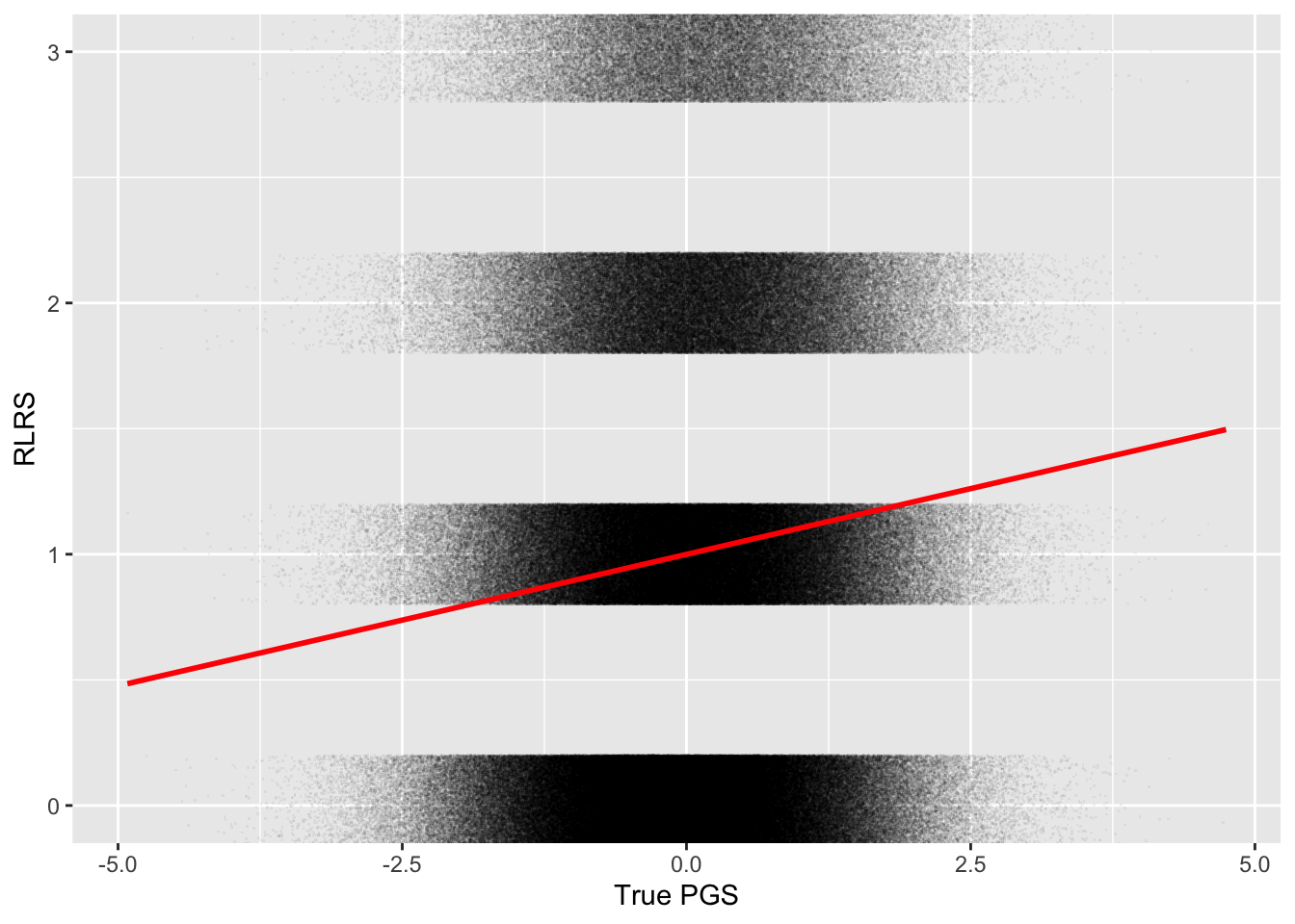
Let’s also simulate data on individuals’ educational attainment. For simplicity I’ll just normalize this to mean 0, variance 1.
# the heritability of EA:
h2 <- 0.45
pop$EA <- faux::rnorm_pre(pop$pgs_true, mu = 0, sd = 1, r = sqrt(h2))
We can check that indeed, the regression of educational attainment on the true PGS gives an r-squared about equal to the heritability:
rsq(EA ~ pgs_true)[1] 0.45PGS with measurement error
Now let’s move into the world of the analyst. We don’t see the true PGS, we just have one measured with error. We can think of it as the true score plus some random noise:
\[ pgs = pgs^* + \eta \]
where \(\eta \sim N(0,\sigma^2_\eta)\). So \(\sigma^2_\eta\) gives the relative amount of error in our measured PGS.
Of course, we don’t see that variable. If so, we could just calculate \(\sigma^2_\eta\) directly by looking at its variance! Instead, we get a standardized PGS with mean 0 variance 1 and we have to estimate how much of that is noise:
\[ pgs = \frac{pgs^* + \eta}{sd(pgs^*)} \]
# this is the variance of the error in measured pgs
# (relative to the true pgs variance of 1)
s2_eta <- 7
pgs <- pop$pgs_true + rnorm(n, 0, sqrt(s2_eta))

# We don't know s2_eta, though we will be able to infer it
# instead we assume the pgs is normalized to variance 1

# This is roughly sqrt(var(pgs_true) + var(eta)) = sqrt(1 + s2_eta)
sd_pgs_orig <- sd(pgs)

pop$pgs <- pgs/sd_pgs_orig
But we can estimate \(\sigma^2_\eta\) by regressing EA on our measured PGS and comparing the r-squared with our prior estimate of the true heritability. This comes from errors-in-variables theory, which gives formulas for the relationship between a regression with a noisy independent variable, and the regression with the true variable. (Here’s a good introduction.)
\[ R^2 (pgs) = R^2 (pgs^*)\times \frac{Var(pgs^*)}{Var(pgs)} \\ = R^2 (pgs^*)\times \frac{1}{1 + \sigma^2_\eta} \]
(There’s a nice proof of this here.)
Rearranging, we can estimate \(\sigma^2_\eta\):
# The R-squared of our measured pgs
r2_EA_pgs <- rsq(EA ~ pgs)

s2_eta_hat <- h2/r2_EA_pgs - 1

s2_eta_hat
[1] 7.01That looks about right. Note that
\[ \hat{\sigma}^2_\eta + 1 = \frac{h^2}{ R^2(pgs) } \]
Now we can estimate the covariance of RLRS and our measured PGS. That will give us the predicted score of our measured PGS in the next generation.
# Now we can estimate the covariance of rlrs and the measured pgs
cov_rlrs_pgs <- cov(pop$rlrs, pop$pgs)
cov_rlrs_pgs
[1] 0.0356# Or equivalently, since the pgs has variance 1
coef_pgs <- coef(lm(rlrs ~ pgs, pop))["pgs"]
coef_pgs pgs
0.0356 # which is close to the average in the next generation:
weighted.mean(pop$pgs, pop$rlrs)[1] 0.0352Compare the plot of measured PGS \(p\) against RLRS to the previous plot, which used the true PGS \(p^*\):
ggplot(pop, aes(pgs, rlrs)) +
  geom_point(alpha = 0.05, pch = ".",
             position = position_jitter(height = 0.2)) +
  geom_smooth(method = "lm", formula = y~x, color = "darkgreen") +
  coord_cartesian(ylim = c(0, 3)) +
  labs(x = "Measured PGS", y = "RLRS")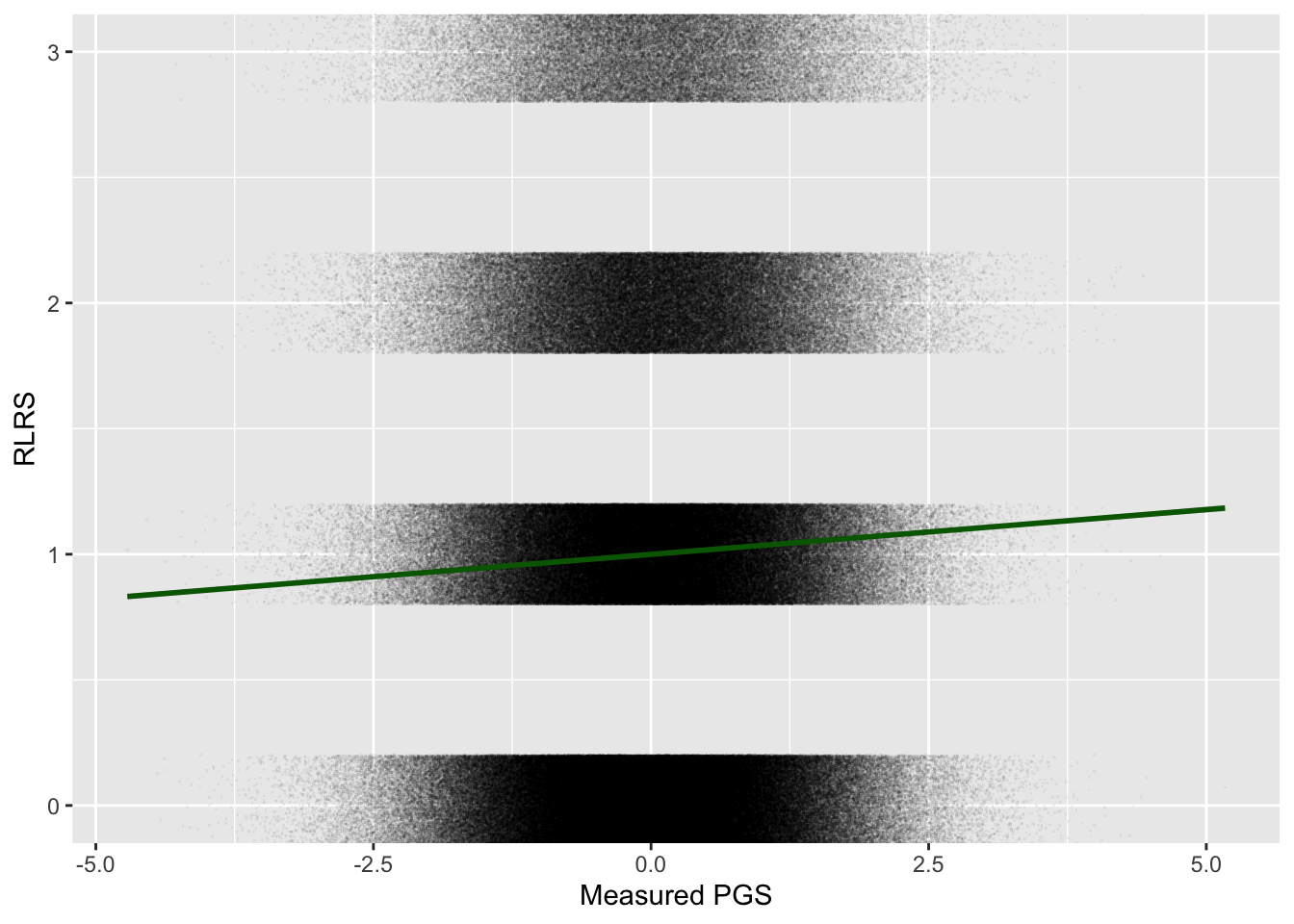
Correcting our estimates
But what we really want to know is the covariance of the true PGS with RLRS. That will give us the average true PGS in the next generation.
To do this, we have to do two things:
Correct the estimate of our regression for the errors-in-variables. We can use our estimate of \(\sigma^2_\eta\) to do that.
Rescale our estimate on to the original scale of the true PGS.
Step 1 again uses the errors-in-variables theory.
\[ \beta_{pgs} = \beta_{pgs^*} \times \frac{Var(pgs^*)}{Var(pgs)} \\ = \beta_{pgs^*} \times \frac{1}{1 + \sigma^2_\eta} \\ \approx \beta_{pgs^*} \times \frac{h^2}{R^2(pgs)} \\ \]
We can check this if we regress RLRS on the true PGS. But we have to rescale the true PGS, the same as we did for the measured PGS, so it is equal to the measured PGS minus error:
pop$pgs_true_rescaled <- pop$pgs_true/sd_pgs_orig

coef_pgs_true_rescaled <- coef(lm(rlrs ~ pgs_true_rescaled, pop))["pgs_true_rescaled"]
coef_pgs_true_rescaled
pgs_true_rescaled
0.296 # Ratio of coefficients...
coef_pgs/coef_pgs_true_rescaled pgs
0.12 # ... is indeed close to ratio of R2 on education, to heritability
r2_EA_pgs/h2[1] 0.125Of course, as analysts, we don’t observe the real rescaled PGS. We can only check this here because we have simulated our data!
Step 2. We want to measure the selection effect of the true PGS in its original form, i.e. with mean 0 and standard deviation 1.
Recall that the measured PGS was “rescaled” by its standard deviation. This standard deviation (sd_pgs_orig in the code above, which equalled 2.828) is the square root of the total variance of the measured PGS on its original scale:
\[ sd(orig. pgs) =\sqrt{1 + \sigma^2_\eta} \]
Again, we have an estimate for this: it is just the square root of \(h^2/R^2(pgs)\).
So, combining steps 1 and 2: we need to multiply our original estimate by \(h^2/R^2(pgs)\) to correct for errors in variables; and divide by \(\sqrt{h^2/R^2(pgs)}\) to rescale. Equivalently, we can just multiply by \(\sqrt{h^2/R^2(pgs)}\) .
cov_rlrs_pgs_true_hat <- cov_rlrs_pgs * sqrt(h2/r2_EA_pgs)

cov_rlrs_pgs_true_hat
[1] 0.101And indeed this is close to the original selection effect of 0.1 .
Assumptions
There are important assumptions here.
Most importantly, the measured PGS is just the true PGS plus random noise. There’s no noise that is correlated with the environment (e.g. with having well-educated parents).
Also, the relationship of the measured PGS with RLRS is entirely driven by the relationship of the true PGS with RLRS. That could be violated if, for example, the measured PGS uses common genetic variants, but among rare unmeasured genetic variants, there is a different relationship between their effect on educational attainment, and their effect on RLRS.
The noise in the measured PGS also doesn’t correlate with RLRS at all.
I’ve ignored epistasis, dominance etc. (Because I don’t really understand them; ask a real geneticist!)
We’re relying a lot on our estimate of heritability.
I haven’t calculated standard errors around the estimate. But we are using estimated statistics in several places (the original coefficient on EA; the coefficient on RLRS; the estimates of heritability…) so we should think carefully about robustness.
Rescaling
Lastly, what if we want to measure the effect of our polygenic score in terms of (e.g.) years of education? Since our estimate is in standard deviations of educational attainment, we just need to rescale it.
sd_ea_years <- 2
# obviously a bit silly, since EA is not normally distributed!
pop$EA_years <- 18 + pop$EA * sd_ea_years

eff_pgs_true <- coef(lm(EA_years ~ pgs_true, pop))["pgs_true"]
pop$pgs_true_years <- pop$pgs_true * eff_pgs_true

# exactly 1
coef(lm(EA_years ~ pgs_true_years, pop))["pgs_true_years"]
pgs_true_years
1 # the selection effect in terms of predicted years of education:
cov(pop$rlrs, pop$pgs_true_years)[1] 0.141weighted.mean(pop$pgs_true_years, pop$rlrs)[1] 0.142# our estimate of the selection effect,
# rescaled by the standard deviation of EA in years:
cov_rlrs_pgs_true_hat * eff_pgs_truepgs_true
0.136 But how do we work out the rescaling factor? We can work it out by taking the square root of the heritability (as an estimate of the effect size of \(pgs^*\) on EA in standard deviations); and multiplying by the s.d. of EA in years (here 2):
eff_pgs_truepgs_true
1.35 sqrt(h2) * sd_ea_years[1] 1.34# selection effect measured in years of education
cov_rlrs_pgs_true_hat * sqrt(h2) * sd_ea_years[1] 0.135Conclusion
I thought this would be useful for anyone who is a statistical schmo like me. For a more rigorous treatment, see e.g. the appendix to Beauchamp (2016); or Becker et al. (2021) here.
You can get the raw code for this document here, and play with the parameters yourself.