Benchmarks

This vignette compares base R and MLX timings across core matrix routines.

library(Rmlx)
#> 
#> Attaching package: 'Rmlx'
#> The following object is masked from 'package:stats':
#> 
#>     fft
#> The following objects are masked from 'package:base':
#> 
#>     asplit, backsolve, chol2inv, col, colMeans, colSums, diag, drop,
#>     outer, row, rowMeans, rowSums, svd
library(bench)
library(ggplot2)

helpers_path <- system.file("benchmarks", "bench_helpers.R", package = "Rmlx")
if (!nzchar(helpers_path)) {
  fallbacks <- c(
    file.path("inst", "benchmarks", "bench_helpers.R"),
    file.path("dev", "benchmarks", "bench_helpers.R")
  )
  helpers_path <- fallbacks[file.exists(fallbacks)][1]
}
if (is.na(helpers_path)) {
  stop("bench_helpers.R not found. Ensure the package is installed or the inst/benchmarks directory is available.")
}
source(helpers_path)

sizes <- c(small = 500L, medium = 1000L, large = 2000L)
inputs <- build_benchmark_inputs(sizes)
operations <- benchmark_operations()

bench_results <- run_benchmarks(operations, inputs)

bench_results$size <- factor(
  bench_results$size,
  levels = names(sizes),
  labels = sizes
)
bench_results$implementation <- factor(
  bench_results$implementation,
  levels = c("base", "mlx"),
  labels = c("base R", "mlx")
)
bench_results$operation <- factor(
  bench_results$operation,
  levels = vapply(operations, `[[`, character(1), "label")
)

ggplot(
  bench_results,
  aes(x = size, y = median_seconds, colour = implementation, group = implementation)
) +
  geom_line() +
  geom_point(size = 2) +
  scale_colour_manual(values = c("base R" = "#4A4A4A", "mlx" = "#D63230")) +
  facet_wrap(~ operation, scales = "free_y") +
  labs(
    title = "Benchmarks for common matrix operations",
    subtitle = "Time taken (less is better)",
    x = "Matrix size",
    y = "Median time (seconds)",
    colour = ""
  ) +
  theme_minimal(base_size = 11) +
  theme(legend.position = "bottom")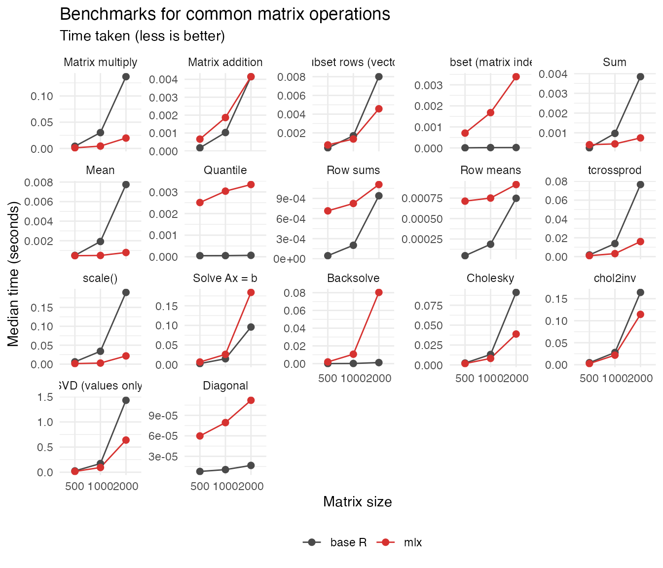

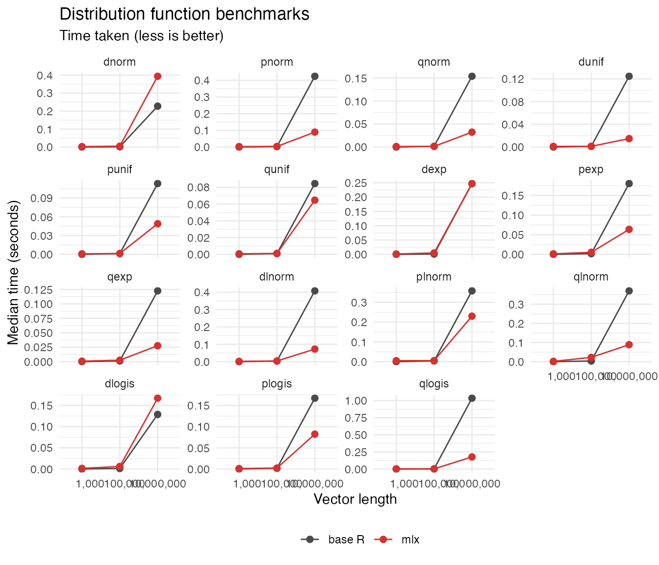
Distribution Functions

Distribution functions operate on vectors rather than matrices, so we benchmark them at larger sizes: 1,000, 100,000, and 10,000,000 elements.

dist_sizes <- c(small = 1000L, medium = 100000L, large = 10000000L)
dist_inputs <- build_distribution_inputs(dist_sizes)
dist_operations <- distribution_operations()

dist_results <- run_benchmarks(dist_operations, dist_inputs)

dist_results$size <- factor(
  dist_results$size,
  levels = names(dist_sizes),
  labels = format(dist_sizes, scientific = FALSE, big.mark = ",")
)
dist_results$implementation <- factor(
  dist_results$implementation,
  levels = c("base", "mlx"),
  labels = c("base R", "mlx")
)
dist_results$operation <- factor(
  dist_results$operation,
  levels = vapply(dist_operations, `[[`, character(1), "label")
)

ggplot(
  dist_results,
  aes(x = size, y = median_seconds, colour = implementation, group = implementation)
) +
  geom_line() +
  geom_point(size = 2) +
  scale_colour_manual(values = c("base R" = "#4A4A4A", "mlx" = "#D63230")) +
  facet_wrap(~ operation, scales = "free_y") +
  labs(
    title = "Distribution function benchmarks",
    subtitle = "Time taken (less is better)",
    x = "Vector length",
    y = "Median time (seconds)",
    colour = ""
  ) +
  theme_minimal(base_size = 11) +
  theme(legend.position = "bottom")