Neural Networks with Rmlx

This vignette demonstrates how to build and train neural networks using Rmlx’s neural network layers and automatic differentiation capabilities.

Building a Neural Network

Rmlx provides modular neural network components that can be combined using mlx_sequential(). Here’s a simple multi-layer perceptron (MLP) for binary classification:

library(Rmlx)
#> 
#> Attaching package: 'Rmlx'
#> The following object is masked from 'package:stats':
#> 
#>     fft
#> The following objects are masked from 'package:base':
#> 
#>     chol2inv, colMeans, colSums, diag, outer, rowMeans, rowSums, svd

# Create a 3-layer MLP
mlp <- mlx_sequential(
  mlx_linear(2, 32),    # Input: 2 features
  mlx_relu(),
  mlx_dropout(p = 0.2),
  mlx_linear(32, 16),
  mlx_relu(),
  mlx_linear(16, 1),    # Output: 1 logit
  mlx_sigmoid()         # Probability output
)

Generating Training Data

Let’s create a simple binary classification dataset:

set.seed(42)

# Generate spiral dataset
n_samples <- 2000
noise <- 0.1

# Class 0: first spiral starting at angle 0
theta0 <- runif(n_samples/2, 0, 4*pi)
r0 <- theta0 / (4*pi) + rnorm(n_samples/2, 0, noise)
x0 <- cbind(r0 * cos(theta0), r0 * sin(theta0))
y0 <- rep(0, n_samples/2)

# Class 1: second spiral starting at angle pi (interleaved)
theta1 <- runif(n_samples/2, 0, 4*pi)
r1 <- theta1 / (4*pi) + rnorm(n_samples/2, 0, noise)
x1 <- cbind(r1 * cos(theta1 + pi), r1 * sin(theta1 + pi))
y1 <- rep(1, n_samples/2)

# Combine
x_train <- rbind(x0, x1)
y_train <- c(y0, y1)

# Convert to MLX tensors
x_mlx <- as_mlx(x_train)
y_mlx <- as_mlx(matrix(y_train, ncol = 1))

# Visualize the training data
plot(x_train[, 1], x_train[, 2],
     col = ifelse(y_train == 0, "blue", "red"),
     pch = 19, cex = 0.8,
     main = "Training Data",
     xlab = "Feature 1", ylab = "Feature 2")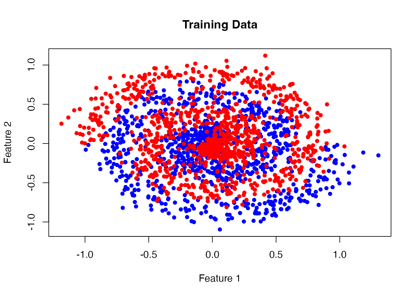

Training Loop

Define a loss function and train using gradient descent:

# Loss function operating on the module
loss_fn <- function(module, x, y) {
  preds <- mlx_forward(module, x)
  mlx_binary_cross_entropy(preds, y)
}

# Training parameters
learning_rate <- 0.05
n_epochs <- 600

# Optimizer and training mode
optimizer <- mlx_optimizer_sgd(mlx_parameters(mlp), lr = learning_rate)
mlx_set_training(mlp, TRUE)

for (epoch in seq_len(n_epochs)) {
  step <- mlx_train_step(mlp, loss_fn, optimizer, x_mlx, y_mlx)

  if (epoch %% 100 == 0) {
    loss_value <- as.numeric(as.matrix(step$loss))
    cat(sprintf("Epoch %d, Loss: %.4f\n", epoch, loss_value))
  }
}
#> Epoch 100, Loss: 0.6639
#> Epoch 200, Loss: 0.6605
#> Epoch 300, Loss: 0.6626
#> Epoch 400, Loss: 0.6577
#> Epoch 500, Loss: 0.6609
#> Epoch 600, Loss: 0.6558

mlx_set_training(mlp, FALSE)

Evaluating Model Performance

Let’s evaluate the model’s predictions:

# Make predictions on all training points
predictions <- mlx_forward(mlp, x_mlx)
pred_probs <- as.matrix(predictions)
pred_classes <- ifelse(pred_probs > 0.5, 1, 0)

# Confusion matrix
confusion <- table(Actual = y_train, Predicted = pred_classes)
print(confusion)
#>       Predicted
#> Actual   0   1
#>      0 771 229
#>      1 544 456

# Calculate accuracy
accuracy <- sum(diag(confusion)) / sum(confusion)
cat(sprintf("\nAccuracy: %.2f%%\n", accuracy * 100))
#> 
#> Accuracy: 61.35%

# Plot predicted classes
plot(x_train[, 1], x_train[, 2],
     col = ifelse(pred_classes == 0, "blue", "red"),
     pch = 19, cex = 0.8,
     main = "Predicted Classes",
     xlab = "Feature 1", ylab = "Feature 2")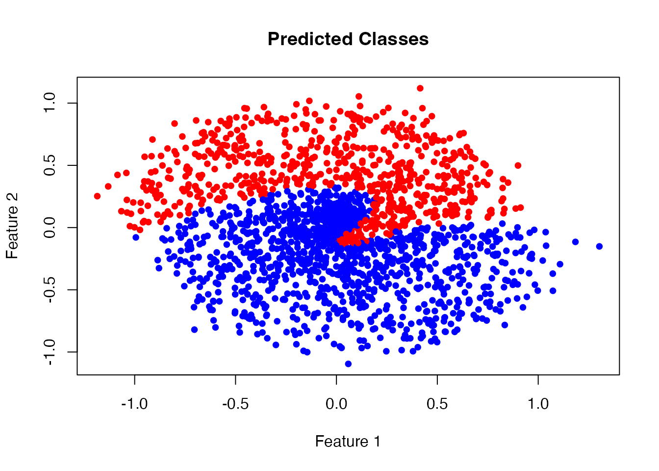

Using Different Architectures

Rmlx provides various layer types for different architectures:

Convolutional Features

While full convolution layers require C++ implementation, you can combine linear layers with reshape operations:

# Classifier with normalization
classifier <- mlx_sequential(
  mlx_linear(10, 64),
  mlx_layer_norm(64),
  mlx_relu(),
  mlx_dropout(p = 0.5),
  mlx_linear(64, 32),
  mlx_batch_norm(32),
  mlx_relu(),
  mlx_linear(32, 3),
  mlx_softmax_layer()  # Multi-class output
)

Embeddings for Categorical Data

Use mlx_embedding() for categorical inputs:

# Text/token embeddings
vocab_size <- 10000
embed_dim <- 128

embedding_net <- mlx_sequential(
  mlx_embedding(vocab_size, embed_dim),
  mlx_linear(embed_dim, 64),
  mlx_relu(),
  mlx_linear(64, 1)
)

# Input: token indices (0-indexed)
tokens <- as_mlx(c(42, 17, 99))
output <- mlx_forward(embedding_net, tokens)

Available Loss Functions

Rmlx implements common loss functions:

mlx_mse_loss(): Mean squared error (regression)
mlx_l1_loss(): Mean absolute error (robust regression)
mlx_binary_cross_entropy(): Binary classification
mlx_cross_entropy(): Multi-class classification

Each supports reduction = "mean", "sum", or "none".

Available Activation Functions

mlx_relu(): Rectified Linear Unit
mlx_gelu(): Gaussian Error Linear Unit
mlx_sigmoid(): Logistic sigmoid
mlx_tanh(): Hyperbolic tangent
mlx_silu(): Sigmoid Linear Unit (Swish)
mlx_leaky_relu(): Leaky ReLU with configurable slope
mlx_softmax_layer(): Softmax normalization

Regularization and Normalization

mlx_dropout(): Dropout regularization
mlx_layer_norm(): Layer normalization
mlx_batch_norm(): Batch normalization

Remember to set training mode appropriately:

model <- mlx_sequential(
  mlx_linear(2, 4),
  mlx_dropout(0.5)
)

# Training
mlx_set_training(model, TRUE)

# Evaluation
mlx_set_training(model, FALSE)

Best Practices

Always evaluate: Call mlx_eval() after parameter updates to trigger computation
Training mode: Set models to training mode during training, evaluation mode during inference
Gradient computation: Use argnums in mlx_grad() to specify which arguments to differentiate
Device management: Ensure all tensors are on the same device (GPU/CPU)