Benchmarks

Setup code

We benchmark RmlxStats against base R and specialized fast fitting packages, across varying numbers of cases (n) and predictors (p). We also check accuracy.

Benchmarking was run on an M2 Macbook Air.

Metadata	Metadata
Generated on	2026-05-22
Commit	03bcaaf
Branch	master
Rmlx version	0.4.0

Benchmarking Code

Data Generation

Code

set.seed(20251111)

n_sizes <- c(10000, 50000, 250000) 
p_sizes <- c(50, 100, 200, 400, 800)
n_max <- max(n_sizes)
p_max <- max(p_sizes)

X <- matrix(rnorm(n_max * p_max), nrow = n_max, ncol = p_max)
colnames(X) <- paste0("x", seq_len(p_max))

X_glmnet <- matrix(rnorm(n_max * p_max), nrow = n_max, ncol = p_max)
for (j in 2:p_max) {
  X_glmnet[, j] <- 0.6 * X_glmnet[, j - 1] + sqrt(1 - 0.6^2) * X_glmnet[, j]
}
colnames(X_glmnet) <- paste0("x", seq_len(p_max))

beta_true <- rnorm(p_max, mean = 0, sd = 0.5)
y_continuous <- drop(X %*% beta_true + rnorm(n_max, sd = 5))

# only 1 in 10 predictors matter:
beta_glmnet_true <- rep(0, p_max)
beta_glmnet_true[seq(10, p_max, 10)] <- rnorm(length(seq(10, p_max, 10)), sd = 0.35)
y_sparse <- drop(X_glmnet %*% beta_glmnet_true + rnorm(n_max, sd = 5))

linpred <- drop(X %*% beta_true) / 10
prob <- 1 / (1 + exp(-linpred))
y_binary <- rbinom(n_max, size = 1, prob = prob)

full_data <- data.frame(
  y_cont = y_continuous,
  y_bin = y_binary,
  y_sparse = y_sparse,
  X
)

# for fast debugging
if (params$develop) {
  n_sizes <- n_sizes/10
  p_sizes <- p_sizes/5
}

bench_grid <- expand.grid(
  n = n_sizes,
  p = p_sizes,
  stringsAsFactors = FALSE
)

bench_grid <- bench_grid[bench_grid$n > bench_grid$p, ]

all_results <- data.frame()
all_accuracy <- data.frame()

Helper functions

relative_rmse <- function(estimate, truth) {
  scale <- sqrt(mean(truth^2))
  sqrt(mean((estimate - truth)^2)) / max(scale, 1e-12)
}

safe_relative_rmse <- function(estimate, truth) {
  estimate <- as.numeric(estimate)
  truth <- as.numeric(truth)

  if (anyNA(estimate) || anyNA(truth) ||
      any(!is.finite(estimate)) || any(!is.finite(truth))) {
    return(NA_real_)
  }

  relative_rmse(estimate, truth)
}

make_pca_fixture <- function(n, p, rank_k, noise_sd = 2) {
  scores_raw <- qr.Q(qr(matrix(rnorm(n * rank_k), nrow = n, ncol = rank_k)))
  scores_raw <- scale(scores_raw, center = TRUE, scale = FALSE)
  scores_basis <- qr.Q(qr(scores_raw))
  rotation <- qr.Q(qr(matrix(rnorm(p * rank_k), nrow = p, ncol = rank_k)))

  sdev_true <- seq(from = 2.5, to = 1.5, length.out = rank_k)
  singular_values <- sdev_true * sqrt(n - 1)
  x_signal <- scores_basis %*% diag(singular_values, nrow = rank_k) %*% 
    t(rotation)
  x <- x_signal + matrix(rnorm(n * p, sd = noise_sd), nrow = n, ncol = p)

  colnames(x) <- paste0("pcx", seq_len(p))

  list(
    x = x,
    rotation = rotation,
    sdev = sdev_true,
    rank = rank_k
  )
}

extract_pca_rotation <- function(fit) {
  if (inherits(fit, "big_SVD")) {
    fit$v
  } else {
    fit$rotation
  }
}

extract_pca_sdev <- function(fit) {
  if (inherits(fit, "big_SVD")) {
    fit$d / sqrt(nrow(fit$u) - 1)
  } else {
    fit$sdev
  }
}

projector_error <- function(estimate, truth) {
  estimate <- as.matrix(estimate)
  truth <- as.matrix(truth)
  proj_estimate <- estimate %*% t(estimate)
  proj_truth <- truth %*% t(truth)
  sqrt(sum((proj_estimate - proj_truth)^2)) / sqrt(sum(proj_truth^2))
}

pca_accuracy_score <- function(fit, truth_rotation, truth_sdev) {
  projector_error(extract_pca_rotation(fit), truth_rotation) +
    relative_rmse(
      as.numeric(extract_pca_sdev(fit)[seq_along(truth_sdev)]),
      truth_sdev
    )
}

make_bootstrap_data <- function(n, p) {
  x <- X[1:n, 1:p, drop = FALSE]
  colnames(x) <- paste0("x", seq_len(p))
  beta <- beta_true[seq_len(p)]
  sigma <- 1 + 2 * abs(x[, 1])
  y <- drop(x %*% beta + rnorm(n, sd = sigma))

  data.frame(y_boot = y, x)
}

bootstrap_oracle_se <- function(x, beta, formula, reps) {
  sigma <- 1 + 2 * abs(x[, 1])
  estimates <- replicate(reps, {
    y <- drop(x %*% beta + rnorm(nrow(x), sd = sigma))
    coef(lm(formula, data = data.frame(y_boot = y, x)))
  })
  apply(t(estimates), 2, sd)
}

extract_bootstrap_se <- function(method, fit) {
  if (identical(method, "stats::lm")) {
    return(as.numeric(fit))
  }

  if (identical(method, "boot::boot")) {
    return(apply(fit$t, 2, sd))
  }

  if (grepl("^lmboot::", method)) {
    return(apply(fit$bootEstParam, 2, sd))
  }

  as.numeric(fit$std.error)
}

mlxs_lm

Code

lm_results <- list()
lm_grid <- bench_grid[bench_grid$n <= n_sizes[2] & bench_grid$p <= p_sizes[3], ]
lm_accuracy <- list()

for (i in seq_len(nrow(lm_grid))) {
  n <- lm_grid$n[i]
  p <- lm_grid$p[i]

  subset_data <- full_data[1:n, c("y_cont", paste0("x", 1:p))]
  lm_formula <- reformulate(paste0("x", 1:p), response = "y_cont")
  beta_target <- beta_true[seq_len(p)]
  fitters <- list(
    "stats::lm" = function() lm(lm_formula, data = subset_data),
    "RmlxStats::mlxs_lm" = function() {
      fit <- mlxs_lm(lm_formula, data = subset_data)
      Rmlx::mlx_eval(fit$coefficients)
      fit
    },
    "fixest::feols" = function() feols(lm_formula, data = subset_data),
    "RcppEigen::fastLm" = function() RcppEigen::fastLm(
      lm_formula,
      data = subset_data
    ),
    "speedglm::speedlm" = function() speedglm::speedlm(
      lm_formula,
      data = subset_data
    )
  )

  bm <- mark(
    "stats::lm" = fitters[["stats::lm"]](),
    "RmlxStats::mlxs_lm" = fitters[["RmlxStats::mlxs_lm"]](),
    "fixest::feols" = fitters[["fixest::feols"]](),
    "RcppEigen::fastLm" = fitters[["RcppEigen::fastLm"]](),
    "speedglm::speedlm" = fitters[["speedglm::speedlm"]](),
    iterations = 3,
    check = function (r1, r2) {
      all.equal(as.vector(coef(r1)), as.vector(coef(r2)), 
                tolerance = 1e-6)
    },
    filter_gc = FALSE
  )

  bm$n <- n
  bm$p <- p
  bm$model_type <- "lm"
  lm_results[[i]] <- bm

  fits <- lapply(fitters, function(fit_method) fit_method())
  scores <- lapply(names(fits), function(method) {
    beta_hat <- as.numeric(coef(fits[[method]]))[-1]
    data.frame(
      model_type = "lm",
      n = n,
      p = p,
      method = method,
      accuracy = relative_rmse(beta_hat, beta_target),
      stringsAsFactors = FALSE
    )
  })
  lm_accuracy[[i]] <- do.call(rbind, scores)
}

lm_df <- do.call(rbind, lm_results)
all_results <- rbind(all_results, lm_df)
all_accuracy <- rbind(all_accuracy, do.call(rbind, lm_accuracy))

mlxs_glm

Code

glm_results <- list()
glm_grid <- bench_grid[bench_grid$n <= n_sizes[2] & bench_grid$p <= p_sizes[3], ]
glm_accuracy <- list()

for (i in seq_len(nrow(glm_grid))) {
  n <- glm_grid$n[i]
  p <- glm_grid$p[i]

  subset_data <- full_data[1:n, c("y_bin", paste0("x", 1:p))]
  glm_formula <- reformulate(paste0("x", 1:p), response = "y_bin")
  beta_target <- beta_true[seq_len(p)] / 5
  fitters <- list(
    "stats::glm" = function() glm(
      glm_formula,
      family = binomial(),
      data = subset_data,
      control = list(maxit = 50)
    ),
    "RmlxStats::mlxs_glm" = function() {
      fit <- mlxs_glm(
        glm_formula,
        family = mlxs_binomial(),
        data = subset_data,
        control = list(maxit = 50, epsilon = 1e-5)
      )
      Rmlx::mlx_eval(fit$coefficients)
      fit
    },
    "speedglm::speedglm" = function() speedglm::speedglm(
      glm_formula,
      family = binomial(),
      data = subset_data
    )
  )

  bm <- mark(
    "stats::glm" = fitters[["stats::glm"]](),
    "RmlxStats::mlxs_glm" = fitters[["RmlxStats::mlxs_glm"]](),
    "speedglm::speedglm" = fitters[["speedglm::speedglm"]](),
    iterations = 3,
    check = function (r1, r2) {
      all.equal(as.vector(coef(r1)), as.vector(coef(r2)), 
                tolerance = 1e-4)
    },
    filter_gc = FALSE
  )

  bm$n <- n
  bm$p <- p
  bm$model_type <- "glm"
  glm_results[[i]] <- bm

  fits <- lapply(fitters, function(fit_method) fit_method())
  scores <- lapply(names(fits), function(method) {
    beta_hat <- as.numeric(coef(fits[[method]]))[-1]
    data.frame(
      model_type = "glm",
      n = n,
      p = p,
      method = method,
      accuracy = relative_rmse(beta_hat, beta_target),
      stringsAsFactors = FALSE
    )
  })
  glm_accuracy[[i]] <- do.call(rbind, scores)
}

glm_df <- do.call(rbind, glm_results)
all_results <- rbind(all_results, glm_df)
all_accuracy <- rbind(all_accuracy, do.call(rbind, glm_accuracy))

mlxs_cv_glmnet

Code

glmnet_results <- list()
glmnet_grid <- bench_grid
glmnet_accuracy <- list()
glmnet_nfolds <- 3L

for (i in seq_len(nrow(glmnet_grid))) {
  n <- glmnet_grid$n[i]
  p <- glmnet_grid$p[i]

  xvars <- paste0("x", 1:p)
  x <- X_glmnet[1:n, xvars, drop = FALSE]
  y_sparse_subset <- y_sparse[1:n]
  beta_target <- beta_glmnet_true[seq_len(p)]
  stats_time <- system.time({
    fit_stats <- glmnet::cv.glmnet(
      x,
      y_sparse_subset,
      nfolds = glmnet_nfolds
    )
    as.numeric(fit_stats$lambda.min)
  })[["elapsed"]]
  mlx_time <- system.time({
    fit_mlx <- mlxs_cv_glmnet(
      x,
      y_sparse_subset,
      nfolds = glmnet_nfolds
    )
    Rmlx::mlx_eval(fit_mlx$glmnet.fit$x_center)
    Rmlx::mlx_eval(fit_mlx$glmnet.fit$x_scale)
    as.numeric(fit_mlx$lambda.min)
  })[["elapsed"]]

  bm <- data.frame(
    expression = c("glmnet::cv.glmnet", "RmlxStats::mlxs_cv_glmnet"),
    median = bench::as_bench_time(c(stats_time, mlx_time)),
    stringsAsFactors = FALSE
  )

  bm$n <- n
  bm$p <- p
  bm$model_type <- "glmnet"
  for (name in setdiff(names(all_results), names(bm))) {
    bm[[name]] <- NA
  }
  bm <- bm[, names(all_results), drop = FALSE]
  glmnet_results[[i]] <- bm

  fits <- list(
    "glmnet::cv.glmnet" = fit_stats,
    "RmlxStats::mlxs_cv_glmnet" = fit_mlx
  )
  scores <- lapply(names(fits), function(method) {
    beta_hat <- as.numeric(coef(fits[[method]], s = "lambda.min"))[-1]
    data.frame(
      model_type = "glmnet",
      n = n,
      p = p,
      method = method,
      accuracy = safe_relative_rmse(beta_hat, beta_target),
      stringsAsFactors = FALSE
    )
  })
  glmnet_accuracy[[i]] <- do.call(rbind, scores)
}

glmnet_df <- do.call(rbind, glmnet_results)
all_results <- rbind(all_results, glmnet_df)
all_accuracy <- rbind(all_accuracy, do.call(rbind, glmnet_accuracy))

mlxs_prcomp

Code

pca_results <- list()
pca_grid <- bench_grid[bench_grid$n <= n_sizes[2] & bench_grid$p <= p_sizes[4], ]
pca_accuracy <- list()

for (i in seq_len(nrow(pca_grid))) {
  n <- pca_grid$n[i]
  p <- pca_grid$p[i]

  rank_k <- min(8L, max(4L, floor(min(n, p) / 2)))
  pca_fixture <- make_pca_fixture(n, p, rank_k)
  x <- pca_fixture$x
  x_big <- bigstatsr::FBM(nrow = n, ncol = p, init = as.matrix(x))
  rotation_true <- pca_fixture$rotation
  fitters <- list(
    "stats::prcomp" = function() prcomp(
      x,
      center = TRUE,
      scale. = FALSE,
      rank. = rank_k
    ),
    "irlba::prcomp_irlba" = function() irlba::prcomp_irlba(
      x,
      n = rank_k,
      center = TRUE,
      scale. = FALSE
    ),
    "rsvd::rpca" = function() rsvd::rpca(
      x,
      k = rank_k,
      center = TRUE,
      scale = FALSE
    ),
    "bigstatsr::big_randomSVD" = function() bigstatsr::big_randomSVD(
      x_big,
      fun.scaling = bigstatsr::big_scale(center = TRUE, scale = FALSE),
      k = rank_k
    ),
    "RmlxStats::mlxs_prcomp" = function() {
      fit <- mlxs_prcomp(
        x,
        center = TRUE,
        scale. = FALSE,
        rank. = rank_k,
        n_iter = 2,
        seed = 1
      )
      Rmlx::mlx_eval(fit$rotation)
      if (!is.null(fit$x)) {
        Rmlx::mlx_eval(fit$x)
      }
      fit
    }
  )

  bm <- mark(
    "stats::prcomp" = fitters[["stats::prcomp"]](),
    "irlba::prcomp_irlba" = fitters[["irlba::prcomp_irlba"]](),
    "rsvd::rpca" = fitters[["rsvd::rpca"]](),
    "bigstatsr::big_randomSVD" = fitters[["bigstatsr::big_randomSVD"]](),
    "RmlxStats::mlxs_prcomp" = fitters[["RmlxStats::mlxs_prcomp"]](),
    iterations = 3,
    check = FALSE,
    filter_gc = FALSE
  )

  bm$n <- n
  bm$p <- p
  bm$model_type <- "pca"
  pca_results[[i]] <- bm

  fits <- lapply(fitters, function(fit_method) fit_method())
  scores <- lapply(names(fits), function(method) {
    data.frame(
      model_type = "pca",
      n = n,
      p = p,
      method = method,
      accuracy = pca_accuracy_score(
        fits[[method]],
        rotation_true,
        pca_fixture$sdev
      ),
      stringsAsFactors = FALSE
    )
  })
  pca_accuracy[[i]] <- do.call(rbind, scores)
}

pca_df <- do.call(rbind, pca_results)
all_results <- rbind(all_results, pca_df)
all_accuracy <- rbind(all_accuracy, do.call(rbind, pca_accuracy))

Bootstrap

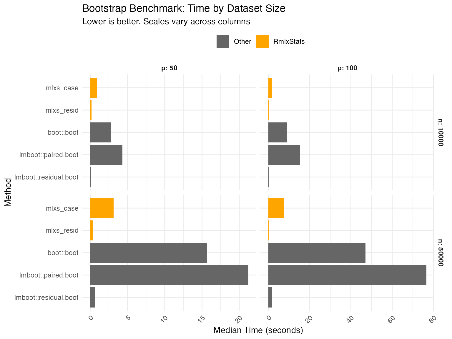
For bootstrap, we use only smaller datasets due to computational cost.

Code

boot_results <- list()
boot_grid <- bench_grid[bench_grid$n <= n_sizes[2] & bench_grid$p <= p_sizes[2], ]
boot_accuracy <- list()
bootstrap_reps <- if (params$develop) 50L else 100L
oracle_reps <- if (params$develop) 50L else 200L

for (i in seq_len(nrow(boot_grid))) {
  n <- boot_grid$n[i]
  p <- boot_grid$p[i]

  subset_data <- make_bootstrap_data(n, p)
  x <- as.matrix(subset_data[paste0("x", seq_len(p))])
  beta_target <- beta_true[seq_len(p)]
  formula_str <- paste("y_boot ~", paste(paste0("x", 1:p), collapse = " + "))
  boot_formula <- as.formula(formula_str)
  fit_mlxs <- mlxs_lm(boot_formula, data = subset_data)
  oracle_se <- bootstrap_oracle_se(x, beta_target, boot_formula, oracle_reps)
  oracle_se <- oracle_se[-1]

  boot_stat <- function(dat, idx) {
    coef(lm(boot_formula, data = dat[idx, , drop = FALSE]))
  }
  fitters <- list(
    "boot::boot" = function() boot::boot(
      subset_data,
      statistic = boot_stat,
      R = bootstrap_reps,
      parallel = "no"
    ),
    "lmboot::paired.boot" = function() lmboot::paired.boot(
      boot_formula,
      data = subset_data,
      B = bootstrap_reps
    ),
    "lmboot::residual.boot" = function() lmboot::residual.boot(
      boot_formula,
      data = subset_data,
      B = bootstrap_reps
    ),
    "mlxs_case" = function() {
      summary(
        fit_mlxs,
        bootstrap = TRUE,
        bootstrap_args = list(
          B = bootstrap_reps,
          seed = 42,
          bootstrap_type = "case",
          progress = FALSE
        )
      )
    },
    "mlxs_resid" = function() {
      summary(
        fit_mlxs,
        bootstrap = TRUE,
        bootstrap_args = list(
          B = bootstrap_reps,
          seed = 42,
          bootstrap_type = "resid",
          progress = FALSE
        )
      )
    }
  )

  bm <- mark(
    "boot::boot" = fitters[["boot::boot"]](),
    "lmboot::paired.boot" = fitters[["lmboot::paired.boot"]](),
    "lmboot::residual.boot" = fitters[["lmboot::residual.boot"]](),
    "mlxs_case" = {
      fit <- fitters[["mlxs_case"]]()
      Rmlx::mlx_eval(fit$std.error)
      fit
    },
    "mlxs_resid" = {
      fit <- fitters[["mlxs_resid"]]()
      Rmlx::mlx_eval(fit$std.error)
      fit
    },
    iterations = 3,
    check = FALSE,
    filter_gc = FALSE,
    memory = FALSE
  )

  bm$n <- n
  bm$p <- p
  bm$model_type <- "Bootstrap"
  boot_results[[i]] <- bm

  fits <- lapply(fitters, function(fit_method) fit_method())
  scores <- lapply(names(fits), function(method) {
    se_hat <- extract_bootstrap_se(method, fits[[method]])[-1]
    data.frame(
      model_type = "Bootstrap",
      n = n,
      p = p,
      method = method,
      accuracy = relative_rmse(se_hat, oracle_se),
      stringsAsFactors = FALSE
    )
  })
  boot_accuracy[[i]] <- do.call(rbind, scores)
}

boot_df <- do.call(rbind, boot_results)
all_results <- rbind(all_results, boot_df)
all_accuracy <- rbind(all_accuracy, do.call(rbind, boot_accuracy))

Results: Speed

We compare functions both against base R implementation, and against the fastest alternative tested.

Display code

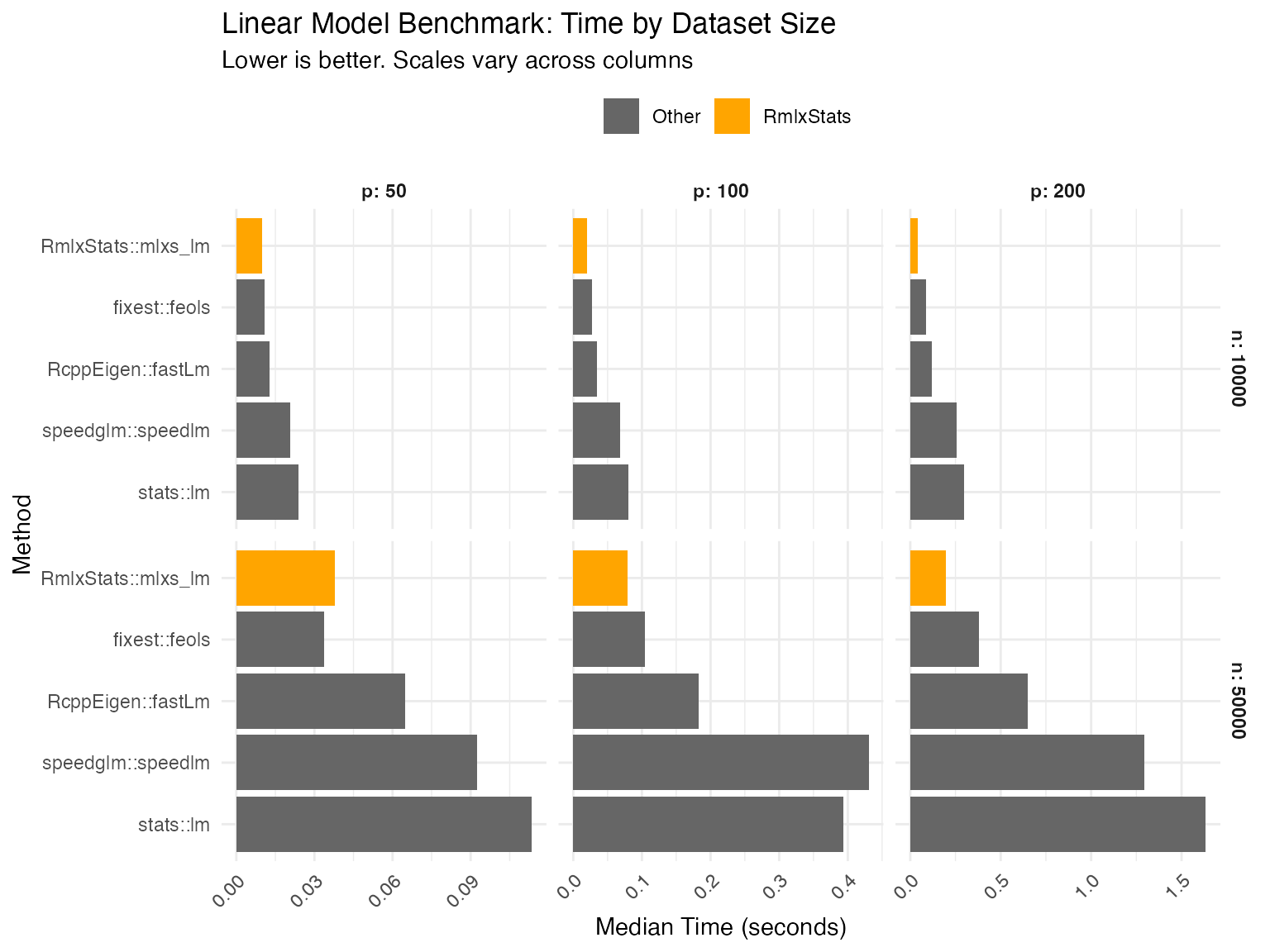
mlxs_lm

Data table

Method	Median seconds	Rel. to base	Rel. to best
n = 10000, p = 50
fixest::feols	0.010	41.5%	100.0%
RcppEigen::fastLm	0.015	59.9%	144.4%
speedglm::speedlm	0.021	85.1%	205.2%
stats::lm	0.025	100.0%	241.0%
RmlxStats::mlxs_lm	0.012	46.2%	111.4%
n = 50000, p = 50
fixest::feols	0.035	29.7%	100.0%
RcppEigen::fastLm	0.088	73.9%	249.1%
speedglm::speedlm	0.11	90.6%	305.1%
stats::lm	0.12	100.0%	336.9%
RmlxStats::mlxs_lm	0.042	34.9%	117.6%
n = 10000, p = 100
fixest::feols	0.028	31.4%	128.1%
RcppEigen::fastLm	0.039	44.8%	182.8%
speedglm::speedlm	0.076	85.8%	350.5%
stats::lm	0.088	100.0%	408.4%
RmlxStats::mlxs_lm	0.022	24.5%	100.0%
n = 50000, p = 100
fixest::feols	0.10	25.1%	100.0%
RcppEigen::fastLm	0.21	51.1%	203.6%
speedglm::speedlm	0.35	84.2%	335.8%
stats::lm	0.41	100.0%	398.8%
RmlxStats::mlxs_lm	0.12	30.2%	120.4%
n = 10000, p = 200
fixest::feols	0.086	28.2%	213.2%
RcppEigen::fastLm	0.12	38.7%	293.3%
speedglm::speedlm	0.26	86.0%	651.0%
stats::lm	0.31	100.0%	756.8%
RmlxStats::mlxs_lm	0.041	13.2%	100.0%
n = 50000, p = 200
fixest::feols	0.40	26.3%	196.2%
RcppEigen::fastLm	0.69	45.3%	337.9%
speedglm::speedlm	1.3	84.4%	629.6%
stats::lm	1.5	100.0%	745.9%
RmlxStats::mlxs_lm	0.21	13.4%	100.0%
Base is base R implementation in 'stats' or 'boot' packages.

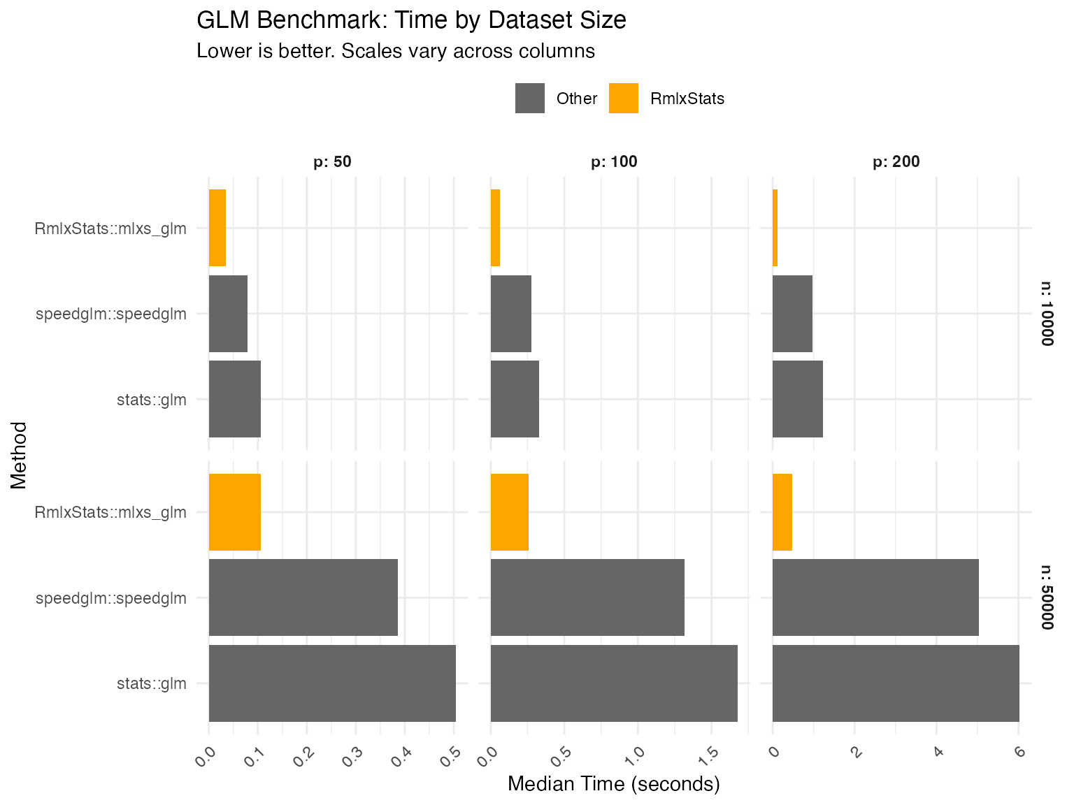
mlxs_glm

Data table

Method	Median seconds	Rel. to base	Rel. to best
n = 10000, p = 50
speedglm::speedglm	0.080	78.0%	152.5%
stats::glm	0.10	100.0%	195.6%
RmlxStats::mlxs_glm	0.052	51.1%	100.0%
n = 50000, p = 50
speedglm::speedglm	0.42	81.0%	254.7%
stats::glm	0.52	100.0%	314.4%
RmlxStats::mlxs_glm	0.16	31.8%	100.0%
n = 10000, p = 100
speedglm::speedglm	0.27	81.1%	369.5%
stats::glm	0.34	100.0%	455.7%
RmlxStats::mlxs_glm	0.074	21.9%	100.0%
n = 50000, p = 100
speedglm::speedglm	1.4	77.0%	436.7%
stats::glm	1.8	100.0%	567.4%
RmlxStats::mlxs_glm	0.31	17.6%	100.0%
n = 10000, p = 200
speedglm::speedglm	1.0	82.5%	726.5%
stats::glm	1.2	100.0%	880.4%
RmlxStats::mlxs_glm	0.14	11.4%	100.0%
n = 50000, p = 200
speedglm::speedglm	5.1	81.9%	791.9%
stats::glm	6.2	100.0%	966.4%
RmlxStats::mlxs_glm	0.64	10.3%	100.0%
Base is base R implementation in 'stats' or 'boot' packages.

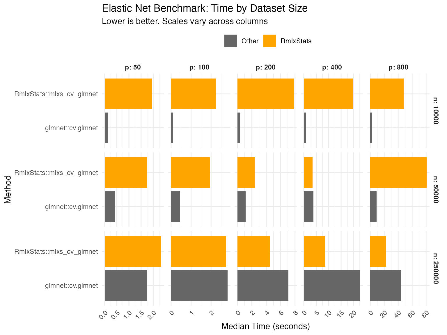
mlxs_cv_glmnet

Data table

Method	Median seconds	Rel. to base	Rel. to best
n = 10000, p = 50
glmnet::cv.glmnet	0.14		100.0%
RmlxStats::mlxs_cv_glmnet	1.9		1348.6%
n = 50000, p = 50
glmnet::cv.glmnet	0.25		100.0%
RmlxStats::mlxs_cv_glmnet	1.7		669.7%
n = 250000, p = 50
glmnet::cv.glmnet	1.8		100.0%
RmlxStats::mlxs_cv_glmnet	1.9		104.7%
n = 10000, p = 100
glmnet::cv.glmnet	0.16		100.0%
RmlxStats::mlxs_cv_glmnet	1.9		1200.0%
n = 50000, p = 100
glmnet::cv.glmnet	0.48		100.0%
RmlxStats::mlxs_cv_glmnet	1.7		358.0%
n = 250000, p = 100
glmnet::cv.glmnet	3.3		127.1%
RmlxStats::mlxs_cv_glmnet	2.6		100.0%
n = 10000, p = 200
glmnet::cv.glmnet	0.25		100.0%
RmlxStats::mlxs_cv_glmnet	6.0		2378.5%
n = 50000, p = 200
glmnet::cv.glmnet	1.4		100.0%
RmlxStats::mlxs_cv_glmnet	2.2		157.2%
n = 250000, p = 200
glmnet::cv.glmnet	7.8		162.4%
RmlxStats::mlxs_cv_glmnet	4.8		100.0%
n = 10000, p = 400
glmnet::cv.glmnet	0.90		100.0%
RmlxStats::mlxs_cv_glmnet	15.		1680.8%
n = 50000, p = 400
glmnet::cv.glmnet	4.5		130.5%
RmlxStats::mlxs_cv_glmnet	3.5		100.0%
n = 250000, p = 400
glmnet::cv.glmnet	34.		120.3%
RmlxStats::mlxs_cv_glmnet	28.		100.0%
n = 10000, p = 800
glmnet::cv.glmnet	3.2		100.0%
RmlxStats::mlxs_cv_glmnet	30.		938.0%
n = 50000, p = 800
glmnet::cv.glmnet	9.3		100.0%
RmlxStats::mlxs_cv_glmnet	54.		586.9%
n = 250000, p = 800
glmnet::cv.glmnet	55.		234.5%
RmlxStats::mlxs_cv_glmnet	23.		100.0%
Base is base R implementation in 'stats' or 'boot' packages.

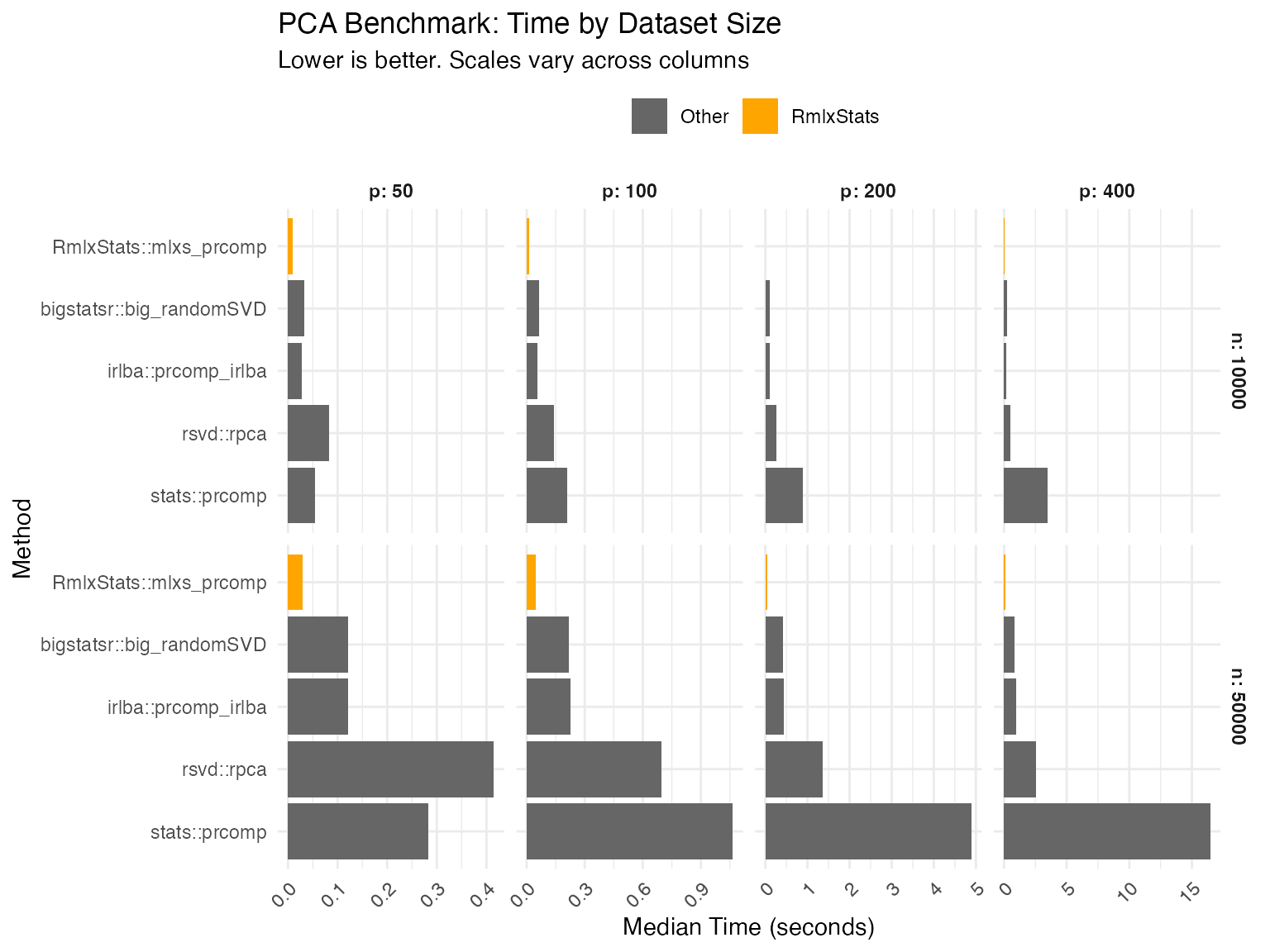
mlxs_prcomp

Data table

Method	Median seconds	Rel. to base	Rel. to best
n = 10000, p = 50
bigstatsr::big_randomSVD	0.033	61.9%	211.5%
irlba::prcomp_irlba	0.031	56.8%	194.2%
rsvd::rpca	0.084	154.7%	529.0%
stats::prcomp	0.054	100.0%	341.9%
RmlxStats::mlxs_prcomp	0.016	29.3%	100.0%
n = 50000, p = 50
bigstatsr::big_randomSVD	0.13	41.6%	588.5%
irlba::prcomp_irlba	0.13	42.7%	604.6%
rsvd::rpca	0.43	141.7%	2006.8%
stats::prcomp	0.30	100.0%	1416.1%
RmlxStats::mlxs_prcomp	0.022	7.1%	100.0%
n = 10000, p = 100
bigstatsr::big_randomSVD	0.053	23.1%	397.5%
irlba::prcomp_irlba	0.057	25.2%	433.0%
rsvd::rpca	0.14	60.0%	1029.7%
stats::prcomp	0.23	100.0%	1717.6%
RmlxStats::mlxs_prcomp	0.013	5.8%	100.0%
n = 50000, p = 100
bigstatsr::big_randomSVD	0.24	21.9%	849.1%
irlba::prcomp_irlba	0.22	20.3%	785.6%
rsvd::rpca	0.74	67.0%	2594.3%
stats::prcomp	1.1	100.0%	3874.0%
RmlxStats::mlxs_prcomp	0.029	2.6%	100.0%
n = 10000, p = 200
bigstatsr::big_randomSVD	0.10	11.6%	645.7%
irlba::prcomp_irlba	0.10	11.5%	641.9%
rsvd::rpca	0.24	26.5%	1473.8%
stats::prcomp	0.90	100.0%	5558.4%
RmlxStats::mlxs_prcomp	0.016	1.8%	100.0%
n = 50000, p = 200
bigstatsr::big_randomSVD	0.43	10.2%	484.9%
irlba::prcomp_irlba	0.49	11.7%	557.2%
rsvd::rpca	1.3	30.9%	1465.7%
stats::prcomp	4.2	100.0%	4746.6%
RmlxStats::mlxs_prcomp	0.088	2.1%	100.0%
n = 10000, p = 400
bigstatsr::big_randomSVD	0.24	6.8%	640.8%
irlba::prcomp_irlba	0.21	6.0%	566.6%
rsvd::rpca	0.49	14.1%	1342.2%
stats::prcomp	3.5	100.0%	9486.5%
RmlxStats::mlxs_prcomp	0.037	1.1%	100.0%
n = 50000, p = 400
bigstatsr::big_randomSVD	0.76	4.6%	793.3%
irlba::prcomp_irlba	0.95	5.8%	990.5%
rsvd::rpca	2.3	13.9%	2368.4%
stats::prcomp	16.	100.0%	17068.6%
RmlxStats::mlxs_prcomp	0.096	0.6%	100.0%
Base is base R implementation in 'stats' or 'boot' packages.

Bootstrap

Data table

Method	Median seconds	Rel. to base	Rel. to best
n = 10000, p = 50
boot::boot	2.9	100.0%	2094.3%
lmboot::paired.boot	4.4	153.9%	3223.2%
lmboot::residual.boot	0.14	4.8%	100.0%
mlxs_case	1.0	36.0%	754.0%
mlxs_resid	0.22	7.7%	161.9%
n = 50000, p = 50
boot::boot	15.	100.0%	3523.0%
lmboot::paired.boot	22.	149.5%	5267.4%
lmboot::residual.boot	0.63	4.2%	147.9%
mlxs_case	3.2	21.6%	759.8%
mlxs_resid	0.43	2.8%	100.0%
n = 10000, p = 100
boot::boot	9.4	100.0%	3670.3%
lmboot::paired.boot	17.	185.1%	6793.4%
lmboot::residual.boot	0.38	4.0%	147.1%
mlxs_case	2.1	22.0%	808.8%
mlxs_resid	0.26	2.7%	100.0%
n = 50000, p = 100
boot::boot	60.	100.0%	10427.6%
lmboot::paired.boot	93.	154.2%	16079.0%
lmboot::residual.boot	1.9	3.2%	333.2%
mlxs_case	20.	33.3%	3467.2%
mlxs_resid	0.58	1.0%	100.0%
Base is base R implementation in 'stats' or 'boot' packages.

Results: Accuracy

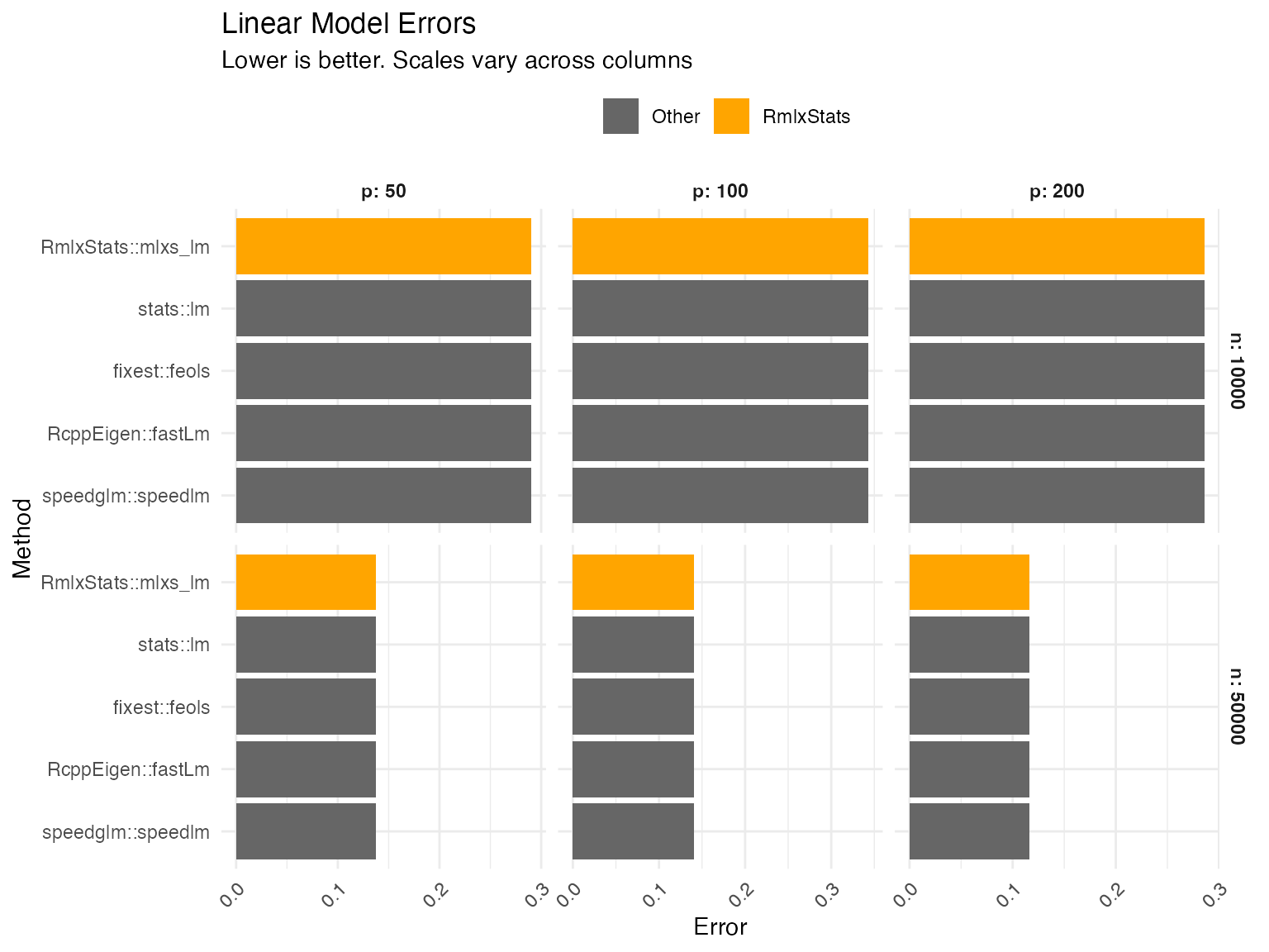
mlxs_lm

Errors are calculated as the relative root mean squared error of the betas (i.e. root mean squared error of the estimated betas compared to the true betas, divided by the root mean square of the true betas).

Data table

Method	Error	Rel. to best
n = 10000, p = 50
stats::lm	0.290	100.0%
RmlxStats::mlxs_lm	0.290	100.0%
fixest::feols	0.290	100.0%
RcppEigen::fastLm	0.290	100.0%
speedglm::speedlm	0.290	100.0%
n = 50000, p = 50
stats::lm	0.137	100.0%
RmlxStats::mlxs_lm	0.137	100.0%
fixest::feols	0.137	100.0%
RcppEigen::fastLm	0.137	100.0%
speedglm::speedlm	0.137	100.0%
n = 10000, p = 100
stats::lm	0.343	100.0%
RmlxStats::mlxs_lm	0.343	100.0%
fixest::feols	0.343	100.0%
RcppEigen::fastLm	0.343	100.0%
speedglm::speedlm	0.343	100.0%
n = 50000, p = 100
stats::lm	0.141	100.0%
RmlxStats::mlxs_lm	0.141	100.0%
fixest::feols	0.141	100.0%
RcppEigen::fastLm	0.141	100.0%
speedglm::speedlm	0.141	100.0%
n = 10000, p = 200
stats::lm	0.286	100.0%
RmlxStats::mlxs_lm	0.286	100.0%
fixest::feols	0.286	100.0%
RcppEigen::fastLm	0.286	100.0%
speedglm::speedlm	0.286	100.0%
n = 50000, p = 200
stats::lm	0.116	100.0%
RmlxStats::mlxs_lm	0.116	100.0%
fixest::feols	0.116	100.0%
RcppEigen::fastLm	0.116	100.0%
speedglm::speedlm	0.116	100.0%

Graph

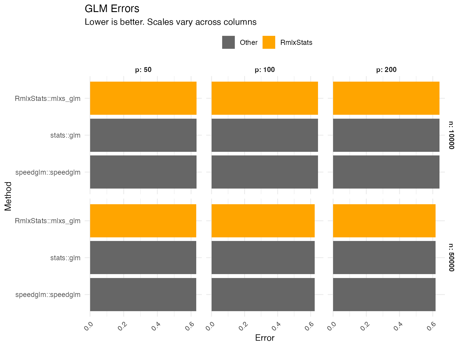
mlxs_glm

Errors are calculated as the relative root mean squared error of the estimated betas.

Data table

Method	Error	Rel. to best
n = 10000, p = 50
stats::glm	0.632	100.0%
RmlxStats::mlxs_glm	0.632	100.0%
speedglm::speedglm	0.632	100.0%
n = 50000, p = 50
stats::glm	0.630	100.0%
RmlxStats::mlxs_glm	0.630	100.0%
speedglm::speedglm	0.630	100.0%
n = 10000, p = 100
stats::glm	0.645	100.0%
RmlxStats::mlxs_glm	0.645	100.0%
speedglm::speedglm	0.645	100.0%
n = 50000, p = 100
stats::glm	0.625	100.0%
RmlxStats::mlxs_glm	0.625	100.0%
speedglm::speedglm	0.625	100.0%
n = 10000, p = 200
stats::glm	0.641	100.0%
RmlxStats::mlxs_glm	0.641	100.0%
speedglm::speedglm	0.641	100.0%
n = 50000, p = 200
stats::glm	0.617	100.0%
RmlxStats::mlxs_glm	0.617	100.0%
speedglm::speedglm	0.617	100.0%

Graph

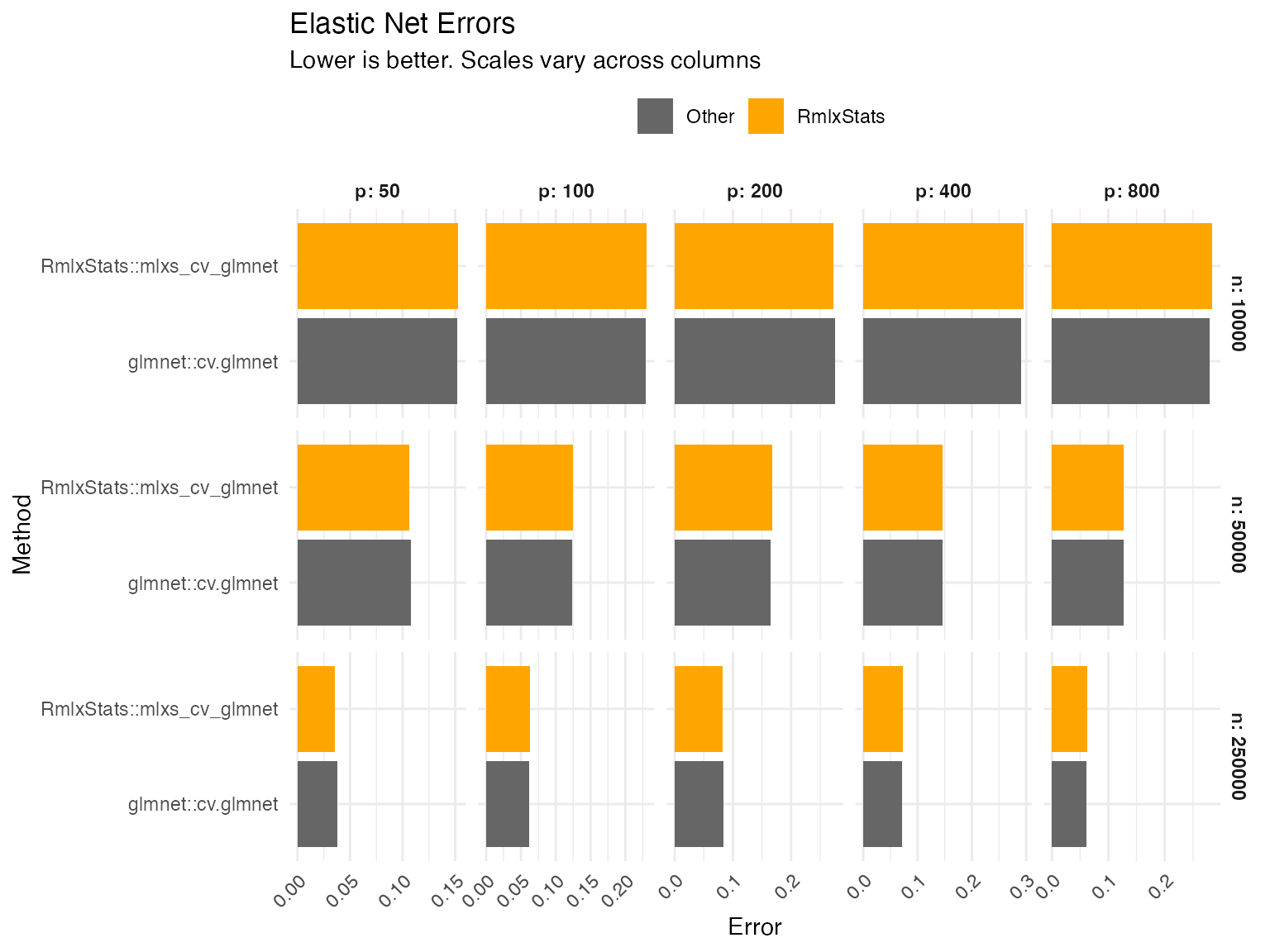
mlxs_cv_glmnet

Errors are calculated as the relative root mean squared error of the estimated betas, for lambda = lambda.min.

Data table

Method	Error	Rel. to best
n = 10000, p = 50
glmnet::cv.glmnet	0.152	100.0%
RmlxStats::mlxs_cv_glmnet	0.153	100.4%
n = 50000, p = 50
glmnet::cv.glmnet	0.108	101.3%
RmlxStats::mlxs_cv_glmnet	0.106	100.0%
n = 250000, p = 50
glmnet::cv.glmnet	0.0375	105.2%
RmlxStats::mlxs_cv_glmnet	0.0357	100.0%
n = 10000, p = 100
glmnet::cv.glmnet	0.229	100.0%
RmlxStats::mlxs_cv_glmnet	0.230	100.6%
n = 50000, p = 100
glmnet::cv.glmnet	0.124	100.0%
RmlxStats::mlxs_cv_glmnet	0.125	100.9%
n = 250000, p = 100
glmnet::cv.glmnet	0.0618	100.0%
RmlxStats::mlxs_cv_glmnet	0.0634	102.6%
n = 10000, p = 200
glmnet::cv.glmnet	0.276	101.2%
RmlxStats::mlxs_cv_glmnet	0.272	100.0%
n = 50000, p = 200
glmnet::cv.glmnet	0.164	100.0%
RmlxStats::mlxs_cv_glmnet	0.168	102.4%
n = 250000, p = 200
glmnet::cv.glmnet	0.0832	101.1%
RmlxStats::mlxs_cv_glmnet	0.0823	100.0%
n = 10000, p = 400
glmnet::cv.glmnet	0.291	100.0%
RmlxStats::mlxs_cv_glmnet	0.296	101.6%
n = 50000, p = 400
glmnet::cv.glmnet	0.147	100.0%
RmlxStats::mlxs_cv_glmnet	0.147	100.0%
n = 250000, p = 400
glmnet::cv.glmnet	0.0713	100.0%
RmlxStats::mlxs_cv_glmnet	0.0731	102.6%
n = 10000, p = 800
glmnet::cv.glmnet	0.280	100.0%
RmlxStats::mlxs_cv_glmnet	0.284	101.8%
n = 50000, p = 800
glmnet::cv.glmnet	0.127	100.0%
RmlxStats::mlxs_cv_glmnet	0.127	100.0%
n = 250000, p = 800
glmnet::cv.glmnet	0.0614	100.0%
RmlxStats::mlxs_cv_glmnet	0.0622	101.3%

Graph

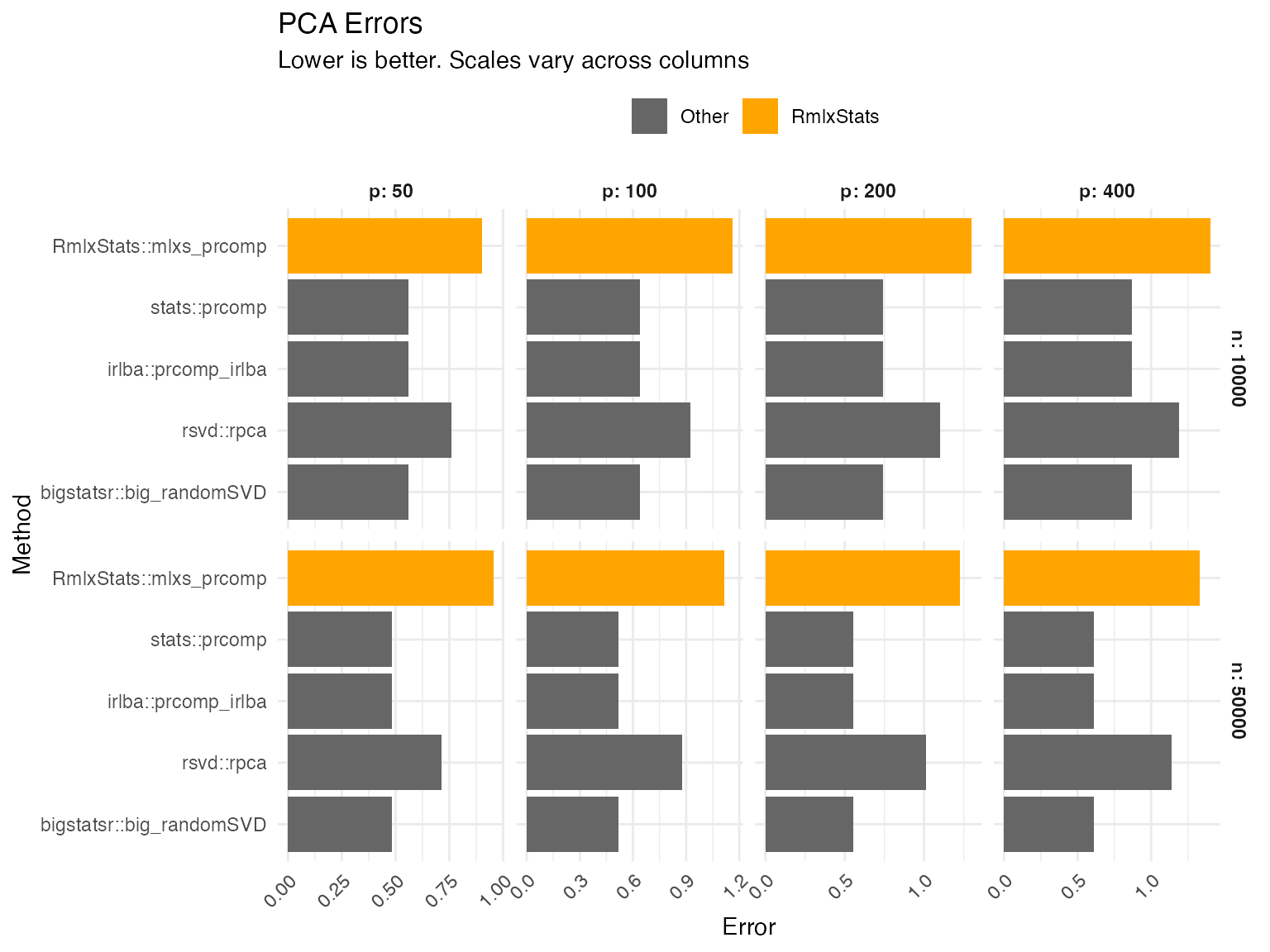
mlxs_prcomp

PCA errors are the projector error of the rotation matrix compared to the true data-generating rotation matrix, plus the relative root mean squared error of the standard deviations. Projector error is equivalent to measuring the principal angles between the estimated and true PCA subspaces.

Data table

Method	Error	Rel. to best
n = 10000, p = 50
stats::prcomp	0.559	100.0%
irlba::prcomp_irlba	0.559	100.0%
rsvd::rpca	0.761	136.2%
bigstatsr::big_randomSVD	0.559	100.0%
RmlxStats::mlxs_prcomp	0.900	161.0%
n = 50000, p = 50
stats::prcomp	0.483	100.0%
irlba::prcomp_irlba	0.483	100.0%
rsvd::rpca	0.712	147.5%
bigstatsr::big_randomSVD	0.483	100.0%
RmlxStats::mlxs_prcomp	0.957	198.4%
n = 10000, p = 100
stats::prcomp	0.642	100.0%
irlba::prcomp_irlba	0.642	100.0%
rsvd::rpca	0.924	144.0%
bigstatsr::big_randomSVD	0.642	100.0%
RmlxStats::mlxs_prcomp	1.16	181.3%
n = 50000, p = 100
stats::prcomp	0.516	100.0%
irlba::prcomp_irlba	0.516	100.0%
rsvd::rpca	0.875	169.6%
bigstatsr::big_randomSVD	0.516	100.0%
RmlxStats::mlxs_prcomp	1.11	215.7%
n = 10000, p = 200
stats::prcomp	0.740	100.0%
irlba::prcomp_irlba	0.740	100.0%
rsvd::rpca	1.10	148.8%
bigstatsr::big_randomSVD	0.740	100.0%
RmlxStats::mlxs_prcomp	1.30	175.5%
n = 50000, p = 200
stats::prcomp	0.552	100.0%
irlba::prcomp_irlba	0.552	100.0%
rsvd::rpca	1.01	183.4%
bigstatsr::big_randomSVD	0.552	100.0%
RmlxStats::mlxs_prcomp	1.23	222.3%
n = 10000, p = 400
stats::prcomp	0.870	100.0%
irlba::prcomp_irlba	0.870	100.0%
rsvd::rpca	1.19	136.7%
bigstatsr::big_randomSVD	0.870	100.0%
RmlxStats::mlxs_prcomp	1.40	161.1%
n = 50000, p = 400
stats::prcomp	0.611	100.0%
irlba::prcomp_irlba	0.611	100.0%
rsvd::rpca	1.14	186.0%
bigstatsr::big_randomSVD	0.611	100.0%
RmlxStats::mlxs_prcomp	1.33	217.6%

Graph

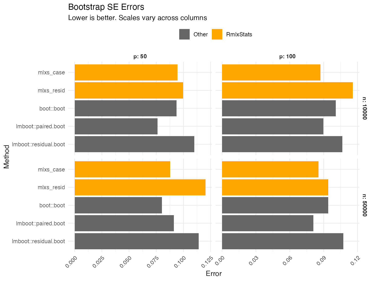
Bootstraps

Errors are calculated as the root mean squared error of the bootstrap-estimated standard errors. We calculate the true standard error by repeatedly estimating linear models, drawing a new dependent variable from the (known) data generating process and calculating the standard deviation of the estimates.

Data table

Method	Error	Rel. to best
n = 10000, p = 50
boot::boot	0.0937	123.0%
lmboot::paired.boot	0.0761	100.0%
lmboot::residual.boot	0.110	144.6%
mlxs_case	0.0945	124.1%
mlxs_resid	0.0997	130.9%
n = 50000, p = 50
boot::boot	0.0803	100.0%
lmboot::paired.boot	0.0912	113.6%
lmboot::residual.boot	0.114	141.9%
mlxs_case	0.0879	109.4%
mlxs_resid	0.120	149.7%
n = 10000, p = 100
boot::boot	0.101	115.7%
lmboot::paired.boot	0.0897	103.0%
lmboot::residual.boot	0.106	122.3%
mlxs_case	0.0870	100.0%
mlxs_resid	0.116	133.1%
n = 50000, p = 100
boot::boot	0.0940	116.1%
lmboot::paired.boot	0.0810	100.0%
lmboot::residual.boot	0.107	132.8%
mlxs_case	0.0854	105.5%
mlxs_resid	0.0940	116.1%

Graph