I have no graphics talent, so this was entirely vibe-coded by Codex. Take it away, Codex!
These examples take familiar R graphics and redraw them through
mypaintr. They use only base R, ggplot2, and
the package itself.
The logo becomes an ink-and-chalk construction rather than a clean vector mark.
Code
{
    par(mar = rep(0, 4), bg = "#f7f8fb")
    plot.new()
    plot.window(c(-5, 5), c(-4, 4), asp = 1)
    outer <- ellipse_xy(-0.4, 0.1, 4.25, 2.45, angle = -0.06)
    inner <- ellipse_xy(-0.35, 0.15, 2.95, 1.45, angle = -0.06)
    set_hand(human_hand(seed = 42, bow = 0.012, wobble = 0.004,
        multi_stroke = 2))
    set_brush("deevad/chalk")
    polygon(outer[, "x"], outer[, "y"], col = "#617493", border = NA)
    set_brush(tweak_brush("tanda/watercolor-02-paint", radius_logarithmic = log(0.8),
        opaque = 0.28, smudge = 0.25, smudge_length = 0.75))
    set_hand(human_hand(seed = 202, bow = 0.01, wobble = 0.004,
        pressure = pressure_smooth(0.55, taper = 0.45)))
    for (yy in seq(-1.8, 1.9, length.out = 9)) {
        lines(c(-3.8, 3.3), c(yy, yy + runif(1, -0.25, 0.25)),
            col = adjustcolor("#7c9ac6", 0.23), lwd = runif(1,
                4, 7))
    }
    set_brush(NULL)
    polygon(inner[, "x"], inner[, "y"], col = "#f7f8fb", border = NA)
    set_brush("classic/textured_ink")
    set_hand(human_hand(seed = 8, bow = 0.006, wobble = 0.003,
        pressure = pressure_smooth(0.75, taper = 0.15)))
    lines(c(-1.8, -1.8, 0.3, 0.95, 0.55, -1.8), c(-1.45, 1.35,
        1.35, 0.72, 0.18, 0.18), col = adjustcolor("#1d3762",
        0.35), lwd = 3.5)
    lines(c(-0.35, 1.45), c(0.08, -1.45), col = adjustcolor("#1d3762",
        0.35), lwd = 3.5)
    set_brush(NULL)
    text(-0.15, -0.32, "R", col = "#17335f", cex = 11.5, font = 2)
    set_brush("experimental/bubble")
    points(runif(70, -3.9, 3.2), runif(70, -2, 2.1), col = adjustcolor("#9fb5d8",
        alpha.f = 0.28), pch = 16, cex = runif(70, 0.4, 1.4))
}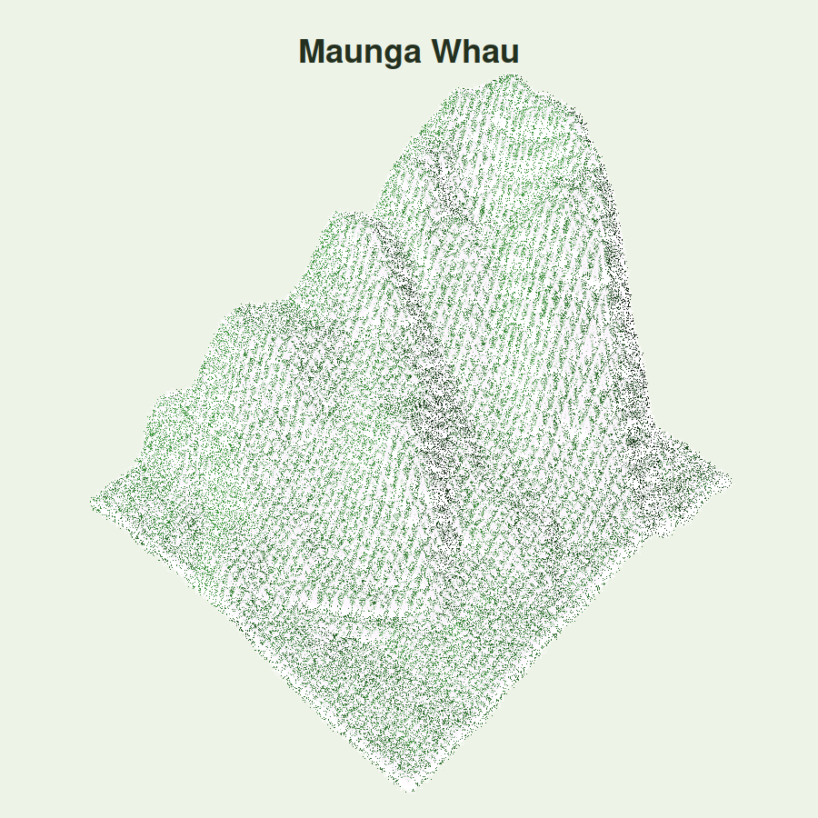
The built-in volcano data rendered as a rough field map.
Code
{
    par(mar = c(0, 0, 0, 0), oma = c(0, 0, 0, 0), bg = "#eef3e8",
        xaxs = "i")
    set_brush(tweak_brush("tanda/charcoal-04", radius_logarithmic = log(0.55),
        opaque = 0.72))
    set_hand(human_hand(seed = 13, bow = 0, wobble = 0.001, pressure = pressure_smooth(0.7,
        taper = 0.25)))
    persp(volcano, phi = 30, theta = 135, shade = 0.55, col = "#3f9c3e",
        border = adjustcolor("white", 0.8), ltheta = 45, box = FALSE,
        axes = FALSE, xlab = "", ylab = "", zlab = "")
    set_brush(NULL)
    mtext("Maunga Whau", side = 3, line = -2.4, col = "#23301f",
        cex = 1.45, font = 2)
}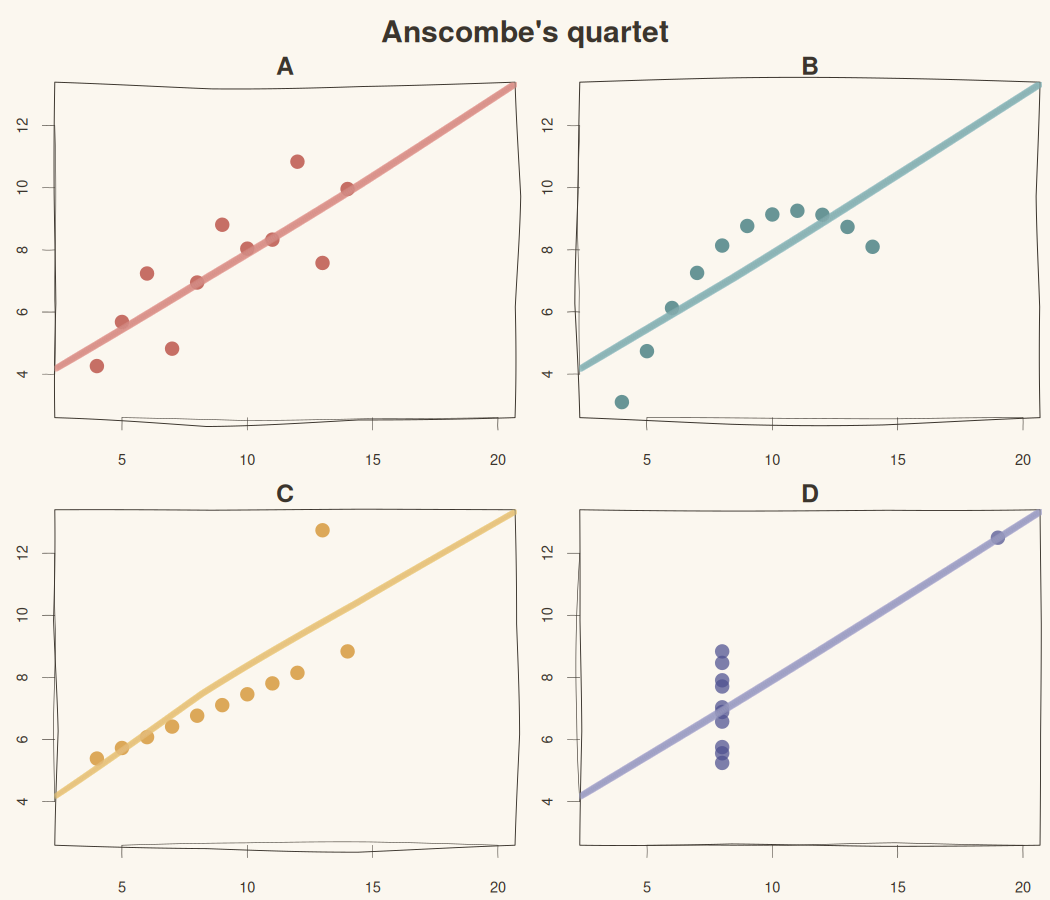
The classic four-panel warning, now with hand-drawn regression lines.
Code
{
    par(mfrow = c(2, 2), mar = c(2.2, 2.2, 1.5, 0.4), oma = c(0,
        0, 1.8, 0), bg = "#fbf7ef")
    cols <- c("#b23a30", "#2f6f73", "#d08a1f", "#4d4f8f")
    set_hand(human_hand(seed = 1, pressure = pressure_smooth(0.6,
        taper = 0.35)))
    for (i in 1:4) {
        x <- anscombe[[paste0("x", i)]]
        y <- anscombe[[paste0("y", i)]]
        set_brush(NULL)
        plot(x, y, xlim = c(3, 20), ylim = c(3, 13), axes = FALSE,
            ann = FALSE, pch = 16, col = adjustcolor(cols[i],
                0.72), cex = 1.55)
        box(col = "#3b352d")
        axis(1, col = "#3b352d", col.axis = "#3b352d", lwd = 0.6,
            cex.axis = 0.7)
        axis(2, col = "#3b352d", col.axis = "#3b352d", lwd = 0.6,
            cex.axis = 0.7)
        set_brush(tweak_brush("classic/slow_ink", radius_logarithmic = log(2),
            opaque = 0.75))
        abline(lm(y ~ x), col = adjustcolor(cols[i], 0.82), lwd = 2)
        set_brush(NULL)
        mtext(LETTERS[i], side = 3, line = 0.2, col = "#3b352d",
            font = 2)
    }
    mtext("Anscombe's quartet", outer = TRUE, cex = 1.2, col = "#3b352d",
        font = 2)
}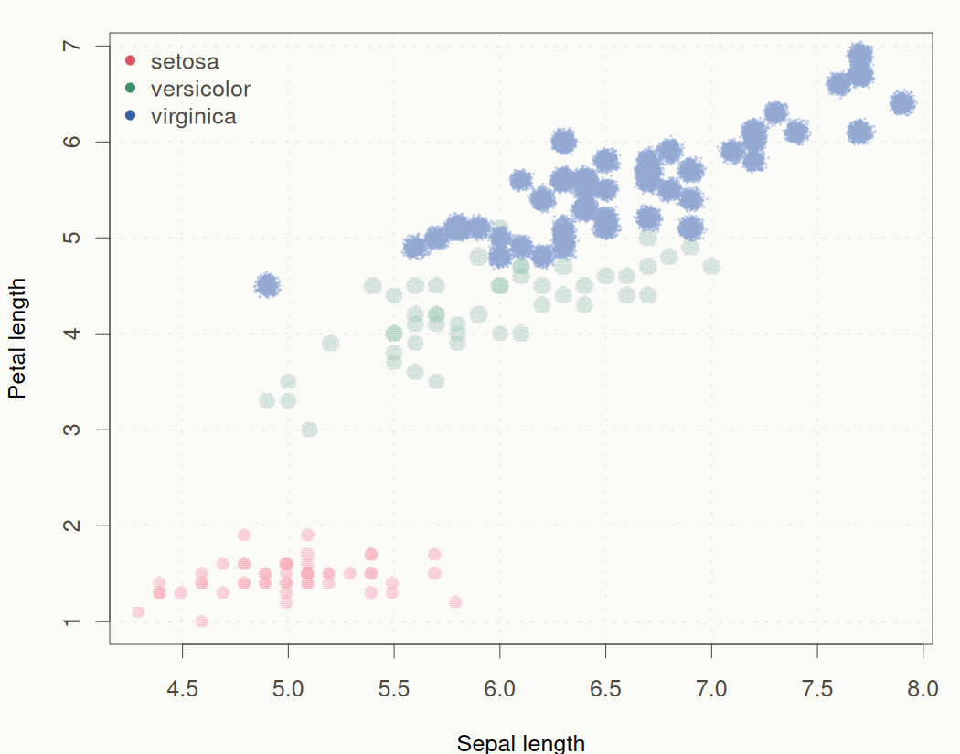
Fisher's iris data as a botanical field-note scatterplot.
Code
{
    par(mar = c(4, 4, 1.2, 1), bg = "#fafaf7")
    set_brush(NULL)
    plot(iris$Sepal.Length, iris$Petal.Length, type = "n", axes = FALSE,
        xlab = "Sepal length", ylab = "Petal length")
    grid(col = "#e7e0d3", lwd = 0.8)
    box(col = "#4a463d")
    axis(1, col = "#4a463d", col.axis = "#4a463d")
    axis(2, col = "#4a463d", col.axis = "#4a463d")
    cols <- c(setosa = "#e05262", versicolor = "#3f8f66", virginica = "#375ca8")
    brushes <- c(setosa = "experimental/bubble", versicolor = "classic/pencil",
        virginica = "deevad/chalk")
    pches <- c(setosa = 24, versicolor = 24, virginica = 16)
    for (sp in levels(iris$Species)) {
        idx <- iris$Species == sp
        set_brush(brushes[[sp]])
        set_hand(hand(pressure = pressure_smooth(0.55, taper = 0.1)))
        points(iris$Sepal.Length[idx], iris$Petal.Length[idx],
            col = adjustcolor(cols[[sp]], 0.78), pch = 16, cex = 1.2 +
                iris$Petal.Width[idx]/3)
    }
    set_brush(NULL)
    legend("topleft", legend = levels(iris$Species), pch = 16,
        col = cols, bty = "n", text.col = "#4a463d")
}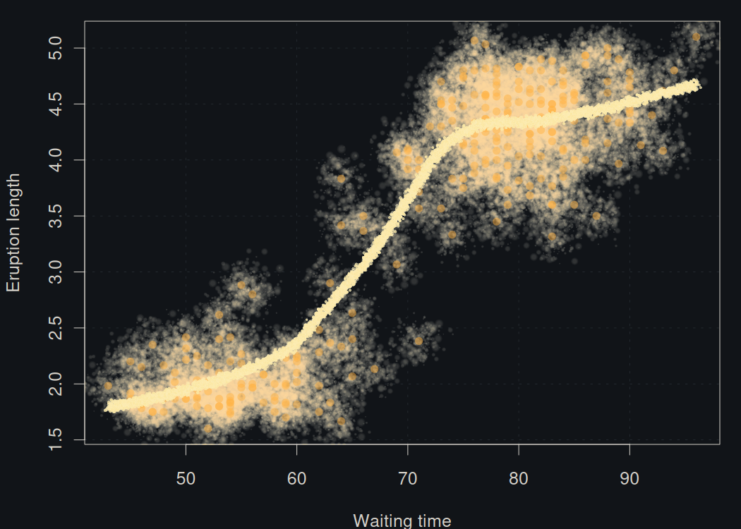
A dark eruption study with a brushed loess curve.
Code
{
    par(mar = c(4, 4, 1, 1), bg = "#111418")
    set_brush(NULL)
    plot(faithful$waiting, faithful$eruptions, type = "n", axes = FALSE,
        xlab = "Waiting time", ylab = "Eruption length", col.lab = "#d5d1c9")
    grid(col = "#2a3138", lwd = 0.7)
    axis(1, col = "#d5d1c9", col.axis = "#d5d1c9")
    axis(2, col = "#d5d1c9", col.axis = "#d5d1c9")
    box(col = "#d5d1c9")
    set_brush("deevad/spray2")
    points(faithful$waiting, faithful$eruptions, col = adjustcolor("#ffb347",
        0.42), pch = 16, cex = 1.4)
    set_brush(NULL)
    points(faithful$waiting, faithful$eruptions, col = adjustcolor("#ffb347",
        0.5), pch = 16)
    set_brush("classic/textured_ink")
    lines(lowess(faithful$waiting, faithful$eruptions, f = 0.45),
        col = adjustcolor("#ffe18a", 0.5), lwd = 1)
}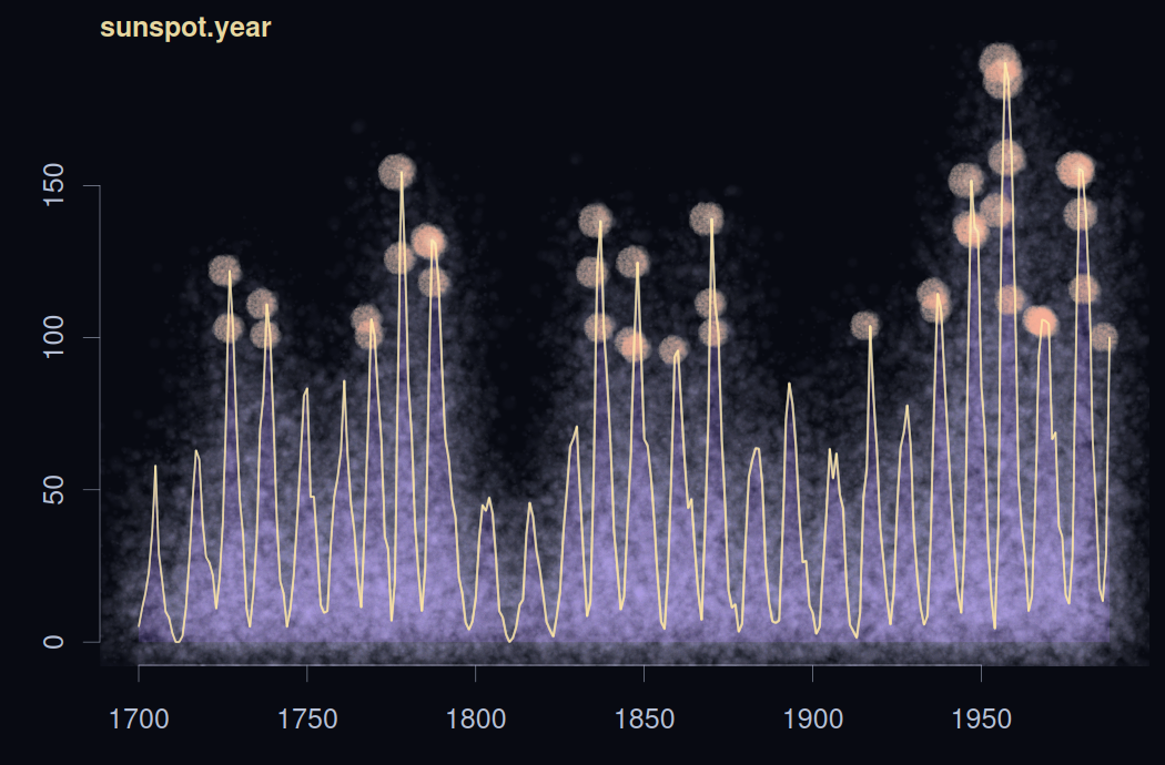
The annual sunspot series treated like an astronomical trace.
Code
{
    par(mar = c(3, 3, 1.2, 0.5), bg = "#080a12")
    y <- as.numeric(sunspot.year)
    years <- as.numeric(time(sunspot.year))
    set_brush(NULL)
    plot(years, y, type = "n", axes = FALSE, ann = FALSE)
    rect(par("usr")[1], par("usr")[3], par("usr")[2], par("usr")[4],
        col = "#080a12", border = NA)
    axis(1, col = "#b7c1d7", col.axis = "#b7c1d7", lwd = 0.5)
    axis(2, col = "#b7c1d7", col.axis = "#b7c1d7", lwd = 0.5)
    mtext("sunspot.year", side = 3, adj = 0, col = "#e7d7a0",
        font = 2)
    set_brush(NULL)
    polygon(c(years, rev(years)), c(rep(0, length(y)), rev(y)),
        col = adjustcolor("#2d1f61", 0.42), border = NA)
    set_brush(tweak_brush("deevad/spray2", radius_logarithmic = log(1.35),
        opaque = 0.62))
    set_hand(hand(pressure = pressure_flat(0.7)))
    segments(years, 0, years, y, col = adjustcolor("#7f62ff",
        0.42), lwd = 2.4)
    peak <- y > 95
    set_brush(tweak_brush("experimental/bubble", radius_logarithmic = log(1.05),
        opaque = 0.75))
    points(years[peak], y[peak], col = adjustcolor("#ff6d3d",
        0.62), pch = 16, cex = 1.2 + y[peak]/95)
    set_brush(tweak_brush("classic/pen", radius_logarithmic = log(0.45),
        opaque = 0.8, dabs_per_actual_radius = 5))
    set_hand(human_hand(seed = 4, pressure = pressure_smooth(0.75,
        taper = 0.45), bow = 0, wobble = 0.001))
    lines(years, y, col = adjustcolor("#ffcc55", 0.95), lwd = 2.2)
    set_brush(tweak_brush("experimental/bubble", radius_logarithmic = log(0.55),
        opaque = 0.7))
    points(years[y > 130], y[y > 130], col = adjustcolor("#fff0a7",
        0.55), pch = 16, cex = 1.1)
}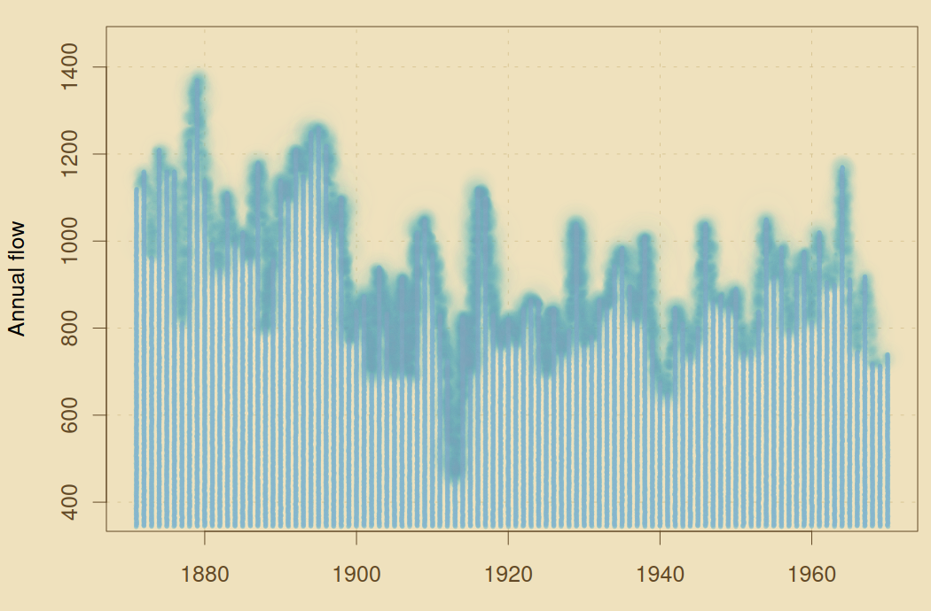
A hydrological time series with papyrus colours and wet ink.
Code
{
    par(mar = c(3, 4, 1, 0.5), bg = "#efe1bd")
    years <- as.numeric(time(Nile))
    flow <- as.numeric(Nile)
    set_brush(NULL)
    plot(years, flow, type = "n", axes = FALSE, xlab = "", ylab = "Annual flow",
        ylim = range(flow) + c(-80, 80))
    rect(par("usr")[1], par("usr")[3], par("usr")[2], par("usr")[4],
        col = "#efe1bd", border = NA)
    grid(col = "#d3be8a", lwd = 0.8)
    axis(1, col = "#614825", col.axis = "#614825")
    axis(2, col = "#614825", col.axis = "#614825")
    box(col = "#614825")
    set_brush("tanda/marker-01")
    segments(years, par("usr")[3] + 10, years, flow, col = adjustcolor("#2879a8",
        0.55), lwd = 1.6)
    set_brush("classic/ink_blot")
    set_hand(human_hand(seed = 71, pressure = pressure_smooth(0.6,
        taper = 0.6)))
    lines(years, flow, col = "#075079", lwd = 3)
}
A simple polar curve turned into a small generative poster.
Code
{
    par(mar = rep(0, 4), bg = "#10100f")
    plot.new()
    plot.window(c(-7, 7), c(-7, 7), asp = 1)
    theta <- seq(0, 9 * pi, length.out = 900)
    r <- seq(0.1, 6.5, length.out = length(theta))
    x <- r * cos(theta)
    y <- r * sin(theta)
    pal <- hcl.colors(9, "Spectral")
    set_hand(human_hand(seed = 100, bow = 0, wobble = 0.0015,
        pressure = pressure_smooth(0.65, taper = 0.65)))
    for (i in seq_len(length(pal))) {
        idx <- seq(floor((i - 1) * length(x)/length(pal)) + 1,
            floor(i * length(x)/length(pal)))
        set_brush(c("classic/pen", "classic/textured_ink", "deevad/chalk")[(i -
            1)%%3 + 1])
        lines(x[idx], y[idx], col = adjustcolor(pal[i], 0.9),
            lwd = 3.3)
    }
    set_brush("experimental/bubble")
    points(x[seq(1, length(x), by = 28)], y[seq(1, length(y),
        by = 28)], col = adjustcolor("#ffffff", 0.22), pch = 16,
        cex = 1.1)
}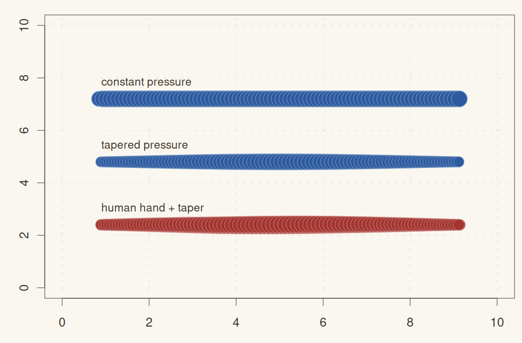
The same stroke logic with constant pressure, tapering, and a human hand.
Code
{
    par(mar = c(3, 3, 1, 0.5), bg = "#faf7f0")
    plot.new()
    plot.window(c(0, 10), c(0, 10))
    set_brush(NULL)
    axis(1, col = "#3d362d", col.axis = "#3d362d")
    axis(2, col = "#3d362d", col.axis = "#3d362d")
    box(col = "#3d362d")
    grid(col = "#e4d7c2")
    set_brush("classic/pen")
    set_hand(hand(pressure = pressure_flat(0.85)))
    lines(c(0.8, 9.2), c(7.2, 7.2), col = "#2c5aa0", lwd = 5)
    set_hand(hand(pressure = pressure_smooth(0.85)))
    lines(c(0.8, 9.2), c(4.8, 4.8), col = "#2c5aa0", lwd = 5)
    set_hand(human_hand(seed = 9, pressure = pressure_smooth(0.85),
        bow = 0.01, wobble = 0.004, multi_stroke = 2))
    lines(c(0.8, 9.2), c(2.4, 2.4), col = "#a3342f", lwd = 5)
    set_brush(NULL)
    text(0.9, c(7.8, 5.4, 3), c("constant pressure", "tapered pressure",
        "human hand + taper"), adj = 0, col = "#3d362d", cex = 0.9)
}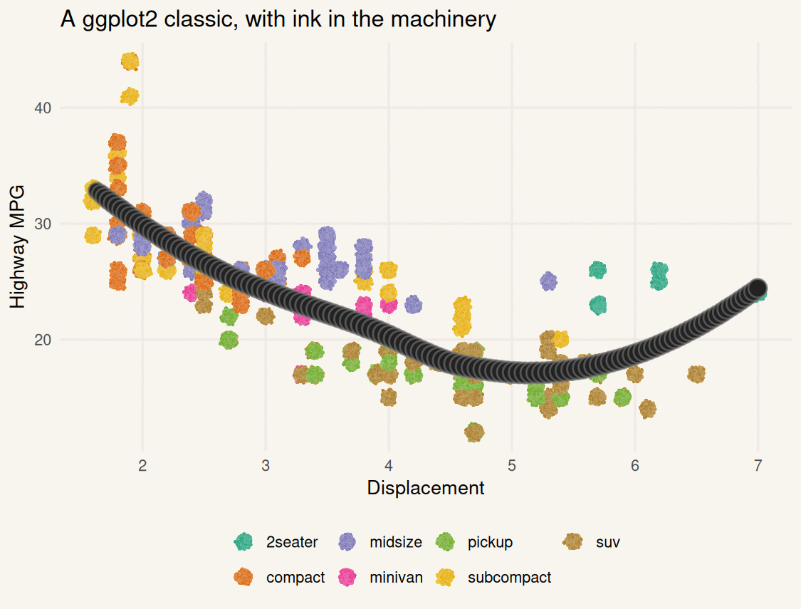
A familiar ggplot scatterplot with mypaintr layers and theme elements.
Code
{
    p <- ggplot(mpg, aes(displ, hwy, colour = class)) + mypaint_wrap(geom_point(size = 2.4,
        alpha = 0.82), brush = "classic/textured_ink", hand = hand(pressure = pressure_smooth(0.6,
        taper = 0.2))) + mypaint_wrap(geom_smooth(aes(group = 1),
        method = "loess", se = FALSE, linewidth = 1.8, colour = "#222222"),
        brush = "classic/slow_ink", hand = human_hand(seed = 2,
            pressure = pressure_smooth(0.7, taper = 0.35))) +
        scale_colour_brewer(palette = "Dark2") + theme_minimal(base_size = 13) +
        theme(panel.grid.major = mypaint_wrap(element_line(colour = "#dad6ca"),
            brush = "classic/pencil"), panel.grid.minor = element_blank(),
            legend.position = "bottom", plot.background = element_rect(fill = "#f8f5ee",
                colour = NA), panel.background = element_rect(fill = "#f8f5ee",
                colour = NA)) + labs(title = "A ggplot2 classic, with ink in the machinery",
        x = "Displacement", y = "Highway MPG", colour = NULL)
    quiet(print(p))
}